Workshop

Supporting Information 1 Organising Reproducible Data Analyses

Emma Rand

17 December, 2024

Introduction

Session overview

In this workshop we will discuss why reproducibility matters and how to organise your work to make it reproducible. We will cover:

What is reproducibility
How to achieve reproducibility
Rationale for scripting
Project-oriented workflow
Code formatting and style
Coding algorithmically
Naming things
And some handy workflow tips

Reproducibility

What is reproducibility?

Two by Two cell matrix. Columns are Data, either same or different. Rows are Analysis either same or different. Each of cells contain one of the definitions for reproducibility — The Turing Way’s definitions of reproducible research

Definitions

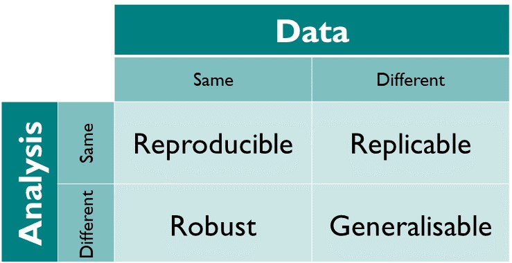
Reproducible: Same data + same analysis = identical results. “… obtaining consistent results using the same input data; computational steps, methods, and code; and conditions of analysis. This definition is synonymous with”computational reproducibility” (National Academies of Sciences et al. 2019). This is what we are concentrating on in the Supporting Information.

Definitions

Replicable: Different data + same analysis = qualitatively similar results. The work is not dependent on the specificities of the data.

Definitions

Robust: Same data + different analysis = qualitatively similar or identical results. The work is not dependent on the specificities of the analysis.

Definitions

Generalisable: Different data + different analysis = qualitatively similar results and same conclusions.

Why does it matter?

Many high profile cases of work which did not reproduce e.g. Anil Potti unravelled by Baggerly and Coombes (2009)
Five selfish reasons to work reproducibly (Markowetz 2015). Alternatively, see the very entertaining talk
Will become standard in Science and publishing e.g OECD Global Science Forum Building digital workforce capacity and skills for data-intensive science (OECD Global Science Forum 2020)

How to achieve reproducibility

Reproducibility is a continuum. Some is better than none!
Script everything
Organisation: Project-oriented workflows with file and folder structure, naming things
Code: follow a consistent style, organise into sections and scripts (be modular), Code algorithmically
Documentation: Readme files, code comments, metadata,
More advanced: version, control, continuous integration and testing (not required for Supporting Information)

Scripting

Rationale for scripting

Science is the generation of ideas, designing work to test them and reporting the results.
We ensure laboratory and field work is replicable, robust and generalisable by planning and recording in lab books and using standard protocols. Repeating results is still hard.
Workflows for computational projects, and the data analysis and reporting of other work can, and should, be 100% reproducible!
Scripting is the way to achieve this.

Organisation of Supporting Information

Project-oriented workflow

use folders to organise your work
you are aiming for structured, systematic and repeatable.
inputs and outputs should be clearly identifiable from structure and/or naming

Example: SI itself is an RSP

-- stem_cell_rna
   |__stem_cell_rna.Rproj   
   |__raw_ data/            
      |__2019-03-21_donor_1.csv
      |__2019-03-21_donor_2.csv
      |__2019-03-21_donor_3.csv
   |__README.md
   |__R/
      |__01_data_processing.R
      |__02_exploratory.R
      |__functions/
         |__theme_volcano.R
         |__normalise.R

Example: SI includes an RSP

-- stem_cell_rna
   |__data_processing/
      |__01_data_processing.py
      |__02_exploratory.py
      |__raw_data/
         |__2019-03-21_donor_1.csv
         |__2019-03-21_donor_2.csv
         |__2019-03-21_donor_3.csv
   |__README.md
   |__statistical_analysis
      |__statistical_analysis.Rproj   
      |__processed_data/
      |__R/
         |__01_DGE.R
         |__02_visualisation.R
         |__functions/
            |__theme_volcano.R
            |__normalise.R

RStudio Projects revisited

RStudio Projects

RStudio Projects make it easy to manage working directories and paths because they set the working directory to the RStudio Projects directory automatically.

RStudio Projects

-- stem_cell_rna
   |__stem_cell_rna.Rproj   
   |__raw_ data/            
      |__2019-03-21_donor_1.csv
   |__README. md
   |__R/
      |__01_data_processing.R
      |__02_exploratory.R
      |__functions/
         |__theme_volcano.R
         |__normalise.R

The project directory is the folder at the top

RStudio Projects

-- stem_cell_rna
   |__stem_cell_rna.Rproj   
   |__raw_ data/            
      |__2019-03-21_donor_1.csv
   |__README. md
   |__R/
      |__01_data_processing.R
      |__02_exploratory.R
      |__functions/
         |__theme_volcano.R
         |__normalise.R

the .RProj file is directly under the project folder¹. Its presence is what makes the folder an RStudio Project

RStudio Projects

When you open an RStudio Project, the working directory is set to the Project directory (i.e., the location of the .Rproj file).
When you use an RStudio Project you do not need to use setwd()
When someone, including future you, opens the project on another machine, all the paths just work.

RStudio Projects

Jenny Bryan

In the words of Jenny Bryan:

“If the first line of your R script is setwd(”C:/Users/jenny/path/that/only/I/have”) I will come into your office and SET YOUR COMPUTER ON FIRE”

Creating an RStudio Project

There are two menus options:

Top left, File menu
Top Right, drop-down indicated by the .RProj icon

They both do the same thing.

Creating an RStudio Project

Then Choose: New Project | New Directory | New Project

Make sure you “Browse” to the folder you want to create the project.

❔ Is your working directory a good place to create a Project folder?

Creating an RStudio Project

When you create a new RStudio Project

A folder called bananas/ is created
RStudio starts a new session in bananas/ i.e., your working directory is now bananas/
A file called bananas.Rproj is created
the .Rproj file is what makes the directory an RStudio Project

Opening and closing

You can close an RStudio Project with ONE of:

File | Close Project
Using the drop-down option on the far right of the tool bar where you see the Project name

Opening and closing

You can open an RStudio Project with ONE of:

File | Open Project or File | Recent Projects
Using the drop-down option on the far right of the tool bar where you see the Project name
Double-clicking an .Rproj file from your file explorer/finder

When you open project, a new R session starts.

Code formatting and style

“Good coding style is like correct punctuation: you can manage without it butitsuremakesthingseasiertoread.”

The tidyverse style guide

Code is not write only.

Code is communication!

Code formatting and style

We have all written code which is hard to read!

We all improve over time.

The only way to write good code is to write tons of shitty code first. Feeling shame about bad code stops you from getting to good code
— Hadley Wickham (@hadleywickham) April 17, 2015

Code formatting and style

Some keys points:

be consistent, emulate experienced coders
use snake_case for variable names (not CamelCase, dot.case)
use <- (not =) for assignment
use spacing around most operators and after commas
use indentation
avoid long lines, break up code blocks with new lines
use " for quoting text (not ') unless the text contains double quotes
space after # for comments

😩 Ugly code 😩

data<-read_csv('../data-raw/Y101_Y102_Y201_Y202_Y101-5.csv',skip=2)
library(janitor);sol<-clean_names(data)
data=data|>filter(str_detect(description,"OS=Homo sapiens"))|>filter(x1pep=='x')
data=data|>
mutate(g=str_extract(description,
"GN=[^\\s]+")|>str_replace("GN=",''))
data<-data|>mutate(id=str_extract(accession,"1::[^;]+")|>str_replace("1::",""))

😩 Ugly code 😩

no spacing or indentation
inconsistent splitting of code blocks over lines
inconsistent use of quote characters
no comments
variable names convey no meaning
use of = for assignment and inconsistently
multiple commands on a line
library statement in the middle of the analysis

😎 Cool code 😎

# Packages ----------------------------------------------------------------
library(tidyverse)
library(janitor)

# Import ------------------------------------------------------------------

# define file name
file <- "../data-raw/Y101_Y102_Y201_Y202_Y101-5.csv"

# import: column headers and data are from row 3
solu_protein <- read_csv(file, skip = 2) |>
  clean_names()

# Tidy data ----------------------------------------------------------------

# filter out the bovine proteins and those proteins 
# identified from fewer than 2 peptides
solu_protein <- solu_protein |>
  filter(str_detect(description, "OS=Homo sapiens")) |>
  filter(x1pep == "x")

# Extract the genename from description column to a column
# of its own
solu_protein <- solu_protein |>
  mutate(genename =  str_extract(description,"GN=[^\\s]+") |>
           str_replace("GN=", ""))

# Extract the top protein identifier from accession column (first
# Uniprot ID after "1::") to a column of its own
solu_protein <- solu_protein |>
  mutate(protid =  str_extract(accession, "1::[^;]+") |>
           str_replace("1::", ""))

😎 Cool code 😎

library() calls collected
Uses code sections to make it easier to navigate
Uses white space and proper indentation
Commented
Uses more informative name for the dataframe

Code ‘algorithmically’

Write code which expresses the structure of the problem/solution.
Avoid hard coding numbers if at all possible - declare variables instead
Declare frequently used values as variables at the start e.g., colour schemes, figure saving settings

😩 Hard coding numbers.

Suppose we want to calculate the sums of squares, \(SS(x)\), for the number of eggs in five nests.
The formula is given by: \(\sum (x_i- \bar{x})^2\)
We could calculate the mean and copy it, and the individual numbers into the formula

😩 Hard coding numbers.

# mean number of eggs per nest
sum(3, 5, 6, 7, 8) / 5

[1] 5.8

# ss(x) of number of eggs
(3 - 5.8)^2 + (5 - 5.8)^2 + (6 - 5.8)^2 + (7 - 5.8)^2 + (8 - 5.8)^2

[1] 14.8

I am coding the calculation of the mean rather using the mean() function only to explain what ‘coding algorithmically’ means using a simple example.

😩 Hard coding numbers

if any of the sample numbers must be altered, all the code needs changing
it is hard to tell that the output of the first line is a mean
its hard to recognise that the numbers in the mean calculation correspond to those in the next calculation
it is hard to tell that 5 is just the number of nests
no way of know if numbers are the same by coincidence or they refer to the same thing

😎 Better

# eggs each nest
eggs <- c(3, 5, 6, 7, 8)

# mean eggs per nest
mean_eggs <- sum(eggs) / length(eggs)

# ss(x) of number of eggs
sum((eggs - mean_eggs)^2)

[1] 14.8

😎 Better

the commenting is similar but it is easier to follow
if any of the sample numbers must be altered, only that number needs changing
assigning a value you will later use to a variable with a meaningful name allows us to understand the first and second calculations
makes use of R’s elementwise calculation which resembles the formula (i.e., is expressed as the general rule)

Naming things

A comic figure is looking over the shoulder of another and is shocked by a list of files with names like 'Untitled 138 copy.docx' and 'Untitled 243.doc'. Caption: 'Protip: Never look in someone else's documents folder' — documents, CC-BY-NC, https://xkcd.com/1459/

Guiding principle - Have a convention! Good file names are:

machine readable
human readable
play nicely with sorting

Naming suggestions

no spaces in names
use snake_case or kebab-case rather than CamelCase or dot.case
use all lower case except very occasionally where convention is otherwise, e.g., README, LICENSE
ordering: use left-padded numbers e.g., 01, 02….99 or 001, 002….999
dates ISO 8601 format: 2020-10-16
write down your conventions

Workflow tips

multiple cursors
open a file/function or find a variable CONTROL+.
the command palette CONTROL+SHIFT+P
segmenting code CONTROL+SHIFT+R
to correct indentation CONTROL+i
to reformat code CONTROL+SHIFT+A Not perfect but corrects spacing, indentation, multiple commands on lines and assignment with =
to comment and uncomment lines CONTROL+SHIFT+C
Tools | Global options | Code | Display | Show margin
Tools | Global options | Code | Diagnostic | Provide R style diagnostics
GitHub Copilot in RStudio, it’s finally here!
It’s all gone wrong, Restart R CONTROL+SHIFT+F10
Fira Code

Summary

Use an RStudio project for any R work (you can also incorporate other languages)
Write Cool code not Ugly code: space, consistency, indentation, comments, meaningful variable names
Write code which expresses the structure of the problem/solution.
Avoid hard coding numbers if at all possible - declare variables instead

Reading

Completely optional suggestions for further reading

Project-oriented workflow | What They Forgot to Teach You About R (Bryan et al., n.d.). Recommended if you still need convincing to use RStudio Projects
Ten simple rules for reproducible computational research (Sandve et al. 2013)
Good enough practices in scientific computing (Wilson et al. 2017)
Excuse Me, Do You Have a Moment to Talk About Version Control? (Bryan 2018)

Pages made with R (R Core Team 2024), Quarto (Allaire et al. 2024), knitr (Xie 2024, 2015, 2014), kableExtra (Zhu 2021)

References

Allaire, J. J., Charles Teague, Carlos Scheidegger, Yihui Xie, and Christophe Dervieux. 2024. “Quarto.” https://doi.org/10.5281/zenodo.5960048.

Baggerly, Keith A, and Kevin R Coombes. 2009. “DERIVING CHEMOSENSITIVITY FROM CELL LINES: FORENSIC BIOINFORMATICS AND REPRODUCIBLE RESEARCH IN HIGH-THROUGHPUT BIOLOGY.” Ann. Appl. Stat. 3 (4): 1309–34. http://www.jstor.org/stable/27801549.

Bryan, Jennifer. 2018. “Excuse Me, Do You Have a Moment to Talk about Version Control?” Am. Stat. 72 (1): 20–27. https://doi.org/10.1080/00031305.2017.1399928.

Bryan, Jennifer, Jim Hester, Shannon Pileggi, and E. David Aja. n.d. What They Forgot to Teach You about r. https://rstats.wtf/.

Markowetz, Florian. 2015. “Five Selfish Reasons to Work Reproducibly.” Genome Biol. 16 (December): 274. https://doi.org/10.1186/s13059-015-0850-7.

National Academies of Sciences, Engineering, Medicine, Policy, Global Affairs, Engineering, Medicine Committee on Science, Public Policy, Board on Research Data, et al. 2019. Understanding Reproducibility and Replicability. National Academies Press (US). https://www.ncbi.nlm.nih.gov/books/NBK547546/.

OECD Global Science Forum. 2020. “Building Digital Workforce Capacity and Skills for Data-Intensive Science.” http://www.oecd.org/officialdocuments/publicdisplaydocumentpdf/?cote=DSTI/STP/GSF(2020)6/FINAL&docLanguage=En.

R Core Team. 2024. R: A Language and Environment for Statistical Computing. Vienna, Austria: R Foundation for Statistical Computing. https://www.R-project.org/.

Sandve, Geir Kjetil, Anton Nekrutenko, James Taylor, and Eivind Hovig. 2013. “Ten Simple Rules for Reproducible Computational Research.” PLoS Comput. Biol. 9 (10): e1003285. https://doi.org/10.1371/journal.pcbi.1003285.

Wilson, Greg, Jennifer Bryan, Karen Cranston, Justin Kitzes, Lex Nederbragt, and Tracy K Teal. 2017. “Good Enough Practices in Scientific Computing.” PLoS Comput. Biol. 13 (6): e1005510. https://doi.org/10.1371/journal.pcbi.1005510.

Xie, Yihui. 2014. “Knitr: A Comprehensive Tool for Reproducible Research in R.” In Implementing Reproducible Computational Research, edited by Victoria Stodden, Friedrich Leisch, and Roger D. Peng. Chapman; Hall/CRC.

———. 2015. Dynamic Documents with R and Knitr. 2nd ed. Boca Raton, Florida: Chapman; Hall/CRC. https://yihui.org/knitr/.

———. 2024. Knitr: A General-Purpose Package for Dynamic Report Generation in r. https://yihui.org/knitr/.

Zhu, Hao. 2021. “kableExtra: Construct Complex Table with ’Kable’ and Pipe Syntax.” https://CRAN.R-project.org/package=kableExtra.

Workshop

Introduction

Session overview

Slide navigation

Reproducibility

What is reproducibility?

Definitions

Definitions

Definitions

Definitions

Why does it matter?

How to achieve reproducibility

Scripting

Rationale for scripting

Organisation of Supporting Information

Project-oriented workflow

Example: SI itself is an RSP

Example: SI includes an RSP

RStudio Projects revisited

RStudio Projects

RStudio Projects

RStudio Projects

RStudio Projects

RStudio Projects

Creating an RStudio Project

Creating an RStudio Project

Creating an RStudio Project

Opening and closing

Opening and closing

Code formatting and style

Code formatting and style

Code formatting and style

Code formatting and style

😩 Ugly code 😩

😩 Ugly code 😩

😎 Cool code 😎

😎 Cool code 😎

Code ‘algorithmically’

Code ‘algorithmically’

😩 Hard coding numbers.

😩 Hard coding numbers.

😩 Hard coding numbers

😎 Better

😎 Better

Naming things

Naming suggestions

Workflow tips

Summary

Reading

References