Independent Study to prepare for workshop
Data Analysis 2: Biomedical sciences - Sample data analysis
Overview
There are three Biomedical Sciences specific data analysis workshops
Week 2 Step-by-step Analysis of sample data
Week 4 Supported Analysis of your own data
Week 6 Customising figures and considering the Class data
Overview
These slides:
Prepare you for the workshop analysing the sample data…. and your own data, which is in the same format
Summarise the experimental design and aims
Explain what the data are
Go through the analytical steps conceptually
Explain what tools we will use in the workshop to do the analysis
Experimental design and aims
Experimental design and aims
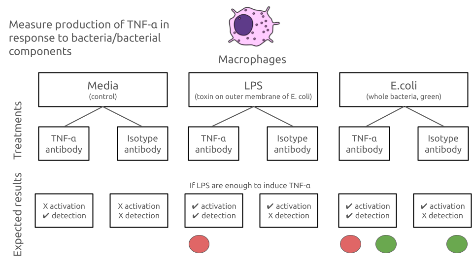
Macrophages produce TNF-α in response to bacterial infection
Question: Does the production of TNF-α by macrophages require live bacteria, or is the cell wall component sufficient?
Therefore we need 3 treatments: Media (control), Lipopolysaccharide (LPS, Cell wall component of E. coli) and live E. coli
We measure TNF-α with a TNF-α antibody conjugated to Allophycocyanin (APC) - this will bind and fluoresce red
Therefore we also need a control for antibody binding and use Isotype antibody - this will bind but not fluoresce
Experimental design and aims
Macrophages are treated with one of three treatments: Media, LPS or NeonGreen fluorescent E.coli
Two antibodies are used for each treatment: Isotype antibody, TNF-α antibody conjugated to Allophycocyanin (APC)
Thus there are 3 x 2 = 6 combinations (i.e., 6 datasets)
Two variables of interest: red fluorescence, green fluorescence
We also measure forward scatter (cell size) and side scatter (cell granularity) which can be used to quality control the cells
Experimental design and aims
We only expect to see red fluorescence (APC) if the treatment induces TNF-α production in macrophages and the TNF-α antibody is used.
We only expect to see green fluorescence (FITC) if the treatment is E. coli
This is summarised in the figure on the next page
Experimental design and aims
The data
The data
The data are in a flow cytometry standard format (FCS) file
Each FCS file contains data from one sample
You will have 6 FCS files, one for each combination of treatment and antibody
There are 16 variables in columns and up to 50000 cells in rows
The data
the 16 columns: TIME, Time MSW, Pulse Width, FS Lin, FS Area, FS Log, SS Lin, SS Area, SS Log, FL 1 Lin, FL 1 Area, FL 1 Log, FL 8 Lin, FL 8 Area, FL 8 Log, Event Count
FS is Forward scatter, SS is Side scatter, FL is fluorescence channel
FL 1 is the green fluorescence channel and we will rename it E_coli_FITC
FL 8 is the red fluorescence channel and we will rename it TNFa_APC
We will use the Lin columns only
We will use just four columns: E_coli_FITC_Lin, TNFa_APC_Lin, FS Lin, and SS Lin
Analytical steps
Overview
The analysis of flow cytometry data is relatively simple conceptually
We apply several quality control steps to the data to remove anomalous signals, dead cells and debris
We use scatter plots, calculate means, and find percentages of cells in different regions of the scatter plots
Analytical steps
Import the data into R and improve the column names
Apply automated quality control
Apply a “logicle” transformation (Parks, Roederer, and Moore 2006) to the fluorescence channels (similar to logging)
Explore the data with scatter plots and histograms/density plots
Use FS Lin and SS Lin to determine what cells (rows) to remove as dead/debris
Determine cut-offs for cells being positive for TNF-α and E. coli
Calculate the percentage of cells that are positive for TNF-α for each treatment combination
Tools
Tools
Import and rename columns using the
flowCorepackage (Ellis et al. 2024)Automated quality control with the
flowAIpackage (Monaco et al. 2016)Apply a “logicle” transformation using the
flowCorepackagePut the data into a dataframe to make it easy to use
tidyverse(Wickham et al. 2019) tools likegroup_by(),summarise(),ggplot(),filter()
The data in R
the
flowCorepackage imports each FCS file as aflowFrameobjectThe
flowFrameobject contains the data from the FCS file and metadata about the experimentA collection of related
flowFramesare stored in aflowSetobjectflowAIandflowCorefunctions work withflowSetobjectsAfter that we can convert the
flowSetto a dataframe to usetidyversetools with which you are more familiar
Summary
Summary
Sample data are like the data you will produce in your own experiment
3 treatments x 2 antibodies = 6 combinations; 4 variables up to 50000 cells each
The analysis is conceptually simple: quality control, transformation, scatter plots, and calculating percentages
The week 2 workshop analyses the sample data, in the week 4 workshop you will analyse your own data
We will use the
flowCore,flowAIandtidyversepackages to do the analysis