Reproducible reports with Quarto

Published

7 April, 2025

Introduction

This workshop introduces you to Quarto (Allaire et al. 2024) for creating reproducible reports.

🎬 An instruction to do something

Learning Outcomes

The successful student will be able to:

explain what Quarto and markdown are
appreciate the role of the YAML header
set default code chunk behaviour and that for individual chunks
use headings, simple text formatting and special characters
add citations and references
use inline code to report results in text
create automatically numbered tables and figures and cross reference them in text

Current process

Typically people analyse, plot and write up in different programs.

90% use Word/Pages/Writer/Googledocs
Updates to data require manual updates to all the figures and tables as well as to text reporting results.
Graphs are saved to files and inserted into the final report.
Reordering figures, tables and equations means updating everywhere they are cross-referenced.
Submitting to a different journal requires reformatting the document.
Manual labour ….. error prone

What is Quarto?

An open-source scientific and technical publishing system that allows you to create dynamic reproducible reports in a variety of output formats.
Next generation RMarkdown. Many new features, greater standardisation and more flexibility.
- Markdown is a lightweight markup language for creating formatted text using a plain-text editor. It was designed by John Gruber in 2004
- RMarkdown is an extension of Markdown that adds support for embedding R code chunks in Markdown documents. It was created by JJ Allaire and Yihui Xie early in 2014 but has been worked on by many others since.
Mutli-language: Python, R, Julia, and Observable.
Include auto-numbered and cross-referencable equations, figures and tables
Integrates with Zotero

Quarto: live demonstration

🎬 Make a copy of the wr-chaff repository:

usethis::use_course("3mmaRand/wr-chaff", destdir = ".")

✔ Downloading from <https://github.com/3mmaRand/wr-chaff/zipball/HEAD>.
Downloaded: 0.73 MB  
✔ Download stored in ./3mmaRand-wr-chaff-3c34954.zip.
✔ Unpacking ZIP file into 3mmaRand-wr-chaff-3c34954/ (61 files extracted).
Shall we delete the ZIP file (3mmaRand-wr-chaff-3c34954.zip)?

1: Definitely
2: Not now
3: No way

🎬 Choose the option that means yes.

Selection: 1
✔ Deleting 3mmaRand-wr-chaff-3c34954.zip.
✔ Opening project in RStudio.

Key points from the demo

Quarto mixes text and code to create dynamic reports
The YAML header sets the default behaviour for the document and is between --- at the top of the document
R Code chunks are between ```{r} and ``` and chunk options, starting #|, determine how/whether they run whether code/output is included in the rendered document
You can run code chunk interactively or through rendering
Comments: |#, # in code chunks,  but use Ctrl+Shift+C

Markdown foundations

Text Formatting

Markdown Syntax	Output
`italics,bold`	italics, bold
`*bold italics *`	*bold italics*
`superscript^2^`	superscript²
`subscript~2~`	subscript₂
`~~strikethrough~~`	~~strikethrough~~
`verbatim code`	`verbatim code`

Headings

Markdown Syntax	Output
`# Header 1`	Header 1
`## Header 2`	Header 2
`### Header 3`	Header 3
`#### Header 4`	Header 4

Links & Images

Markdown Syntax	Output
`[Quar to](https://quarto.org)`	Quarto
`![Cap tion](images/chaff.jpg)`	Caption

Equations

Use $ delimiters for inline maths and $$ delimiters for display maths. For example:

Markdown Syntax Output

Markdown Syntax	Output
`i nline maths: $E = mc^{2}$`	inline maths: \(E=mc^{2}\)
`display maths: $$E = mc^{2}$$`	display maths: \[E = mc^{2}\]

i
nline maths: $E = mc^{2}$

inline maths: $E=mc^{2}$

display maths:

$$E = mc^{2}$$

display maths:

\[E = mc^{2}\]

Divs

“Divs” are used to group content together. They can be used to apply styling to that content.

We also use them for grouping a code chunks with text. This is useful for creating multi-panel figures with legends.

Create your own Quarto document

Create a new project

🎬 File | New Project | New Directory | Quarto Project

Browse to an appropriate place and give your project a name.
I used wr-chaff
Choose Engine: Knitr
Turn visual markdown editor off (for now)

Change some RStudio settings

🎬 Tools | Global Options

General:
- Turn off the three “Restore ….” options
- Turn “Save workspace to .RData on exit” to Never
R Markdown:
- Turn “Show output preview in:” to Viewer pane

Your project contains

wr-chaff.RProj - what makes the folder an RStudio project
_quarto.yml - the configuration file
wr-chaff.md - the main document containing some template text

🎬 Hit Render (Ctrl-Shift-K)

Note that wr-chaff.html is created and opened in the Viewer pane

Edit the YAML header

🎬 Add your name, and a title. Also add the engine and format

---
title: "The difference in mass between subspecies of common chaffinch."
author: "Emma Rand"
engine: knitr
format:
  html
---

Add some content

🎬 Add a code chunk (Ctrl-Shift-I) for a simple graph.

```{r}
hist(rnorm(100))
```

🎬 Hit Render (Ctrl-Shift-K)

Edit the YAML header: default code chunk options

🎬 Set some default code chunk options. I recommend these for reports

---
title: "The difference in mass between subspecies of common chaffinch."
author: "Emma Rand"
engine: knitr
format:
  html
execute:
  echo: false
  include: true
  error: false
  message: false
  warning: false

---

🎬 Hit Render (Ctrl-Shift-K)

Code chunk options

echo: false code will not be included in output
include: true output will be included
error: false halt render if a code error occurs
message: false messages and warnings will not be included
warning: false

🎬 Experiment with change the options and re-rendering. Try misspelling rnorm to see the error option in action.

Adding content

🎬 Delete everything except the YAML header.

🎬 Add headings for: Introduction, Methods, Results, Discussion, and References

🎬 Add a code chunk for package loading

```{r}
#| label: load-packages
library(tidyverse)
```

#| label: load-packages is a code chunk label. These are useful (here) and essential (later) for cross-referencing.

An Introduction

🎬 Add this test to the Introduction

A number of subspecies of the common chaffinch, Fringilla coelebs, have been described based principally on the differences in the pattern and colour of the adult male plumage. Two of groups of these subspecies are the “coelebs group” that occurs in Europe and Asia and the “canariensis group” that occurs on the Canary Islands.

🎬 Make the species name italic

🎬 Make “common chaffinch” a link to https://en.wikipedia.org/wiki/Common_chaffinch

Data import

🎬 Make a folder called data-raw

🎬 Save chaff.txt to data-raw

🎬 Add a code chunk with:

```{r}
#| label: import-data
file <- "data-raw/chaff.txt"
chaff <- read_table(file)
```

🎬 Run chunks interactively

🎬 Render

Data summary

🎬 Add a code chunk with:

```{r}
#| label: data-summary
chaff_summary <- chaff |> 
  group_by(subspecies) |>  
  summarise(mean = mean(mass, na.rm = TRUE),
            sd = sd(mass, na.rm = TRUE),
            n = length(mass),
            se = sd / sqrt(n))
```

🎬 Render

Notice the chunk labels being used in “Background Jobs”

Methods text

🎬 Add this text to Methods:

We randomly sampled 20 F. c. coelebs males and 20 F. c. palmae males and determined their mass with spring scales. Analysis was carried out with R and tidyverse packages.

It would be good not to have “hard coded” those numbers in the text. What if we get more data. Or we just misremember or mis-type the numbers?

Inline code: reproducible reporting

Inline code is how you include a variable value, like a sample size, mean or statistical result, in a section of text.
In fact, any code output can be inserted directly into the text of a .qmd file using inline code.

Inline code goes between `r` and ` .

For example by writing:

The squareroot of 2 is `r sqrt(2) `

you will get:

The squareroot of 2 is 1.4142136

Extract summary information for use in inline code

🎬 Add a code chunk with:

```{r}
#| label: extract-summary
# extract values for inline reporting

# sample sizes
n_coelebs <- chaff_summary |> 
  filter(subspecies == "coelebs") |> 
  pull(n)

n_canariensis <- chaff_summary |> 
  filter(subspecies == "canariensis") |> 
  pull(n)
```

🎬 Replace the sample sizes in the Methods text with inline code

🎬 Render

Figures

🎬 Add a code chunk to the Results section with:

```{r}
#| label: fig-chaff
ggplot() +
  geom_point(data = chaff, aes(x = subspecies, y = mass),
             position = position_jitter(width = 0.1, height = 0),
             colour = "gray50") +
  geom_errorbar(data = chaff_summary, 
                aes(x = subspecies, ymin = mean - se, ymax = mean + se),
                width = 0.3) +
  geom_errorbar(data = chaff_summary, 
                aes(x = subspecies, ymin = mean, ymax = mean),
                width = 0.2) +
  scale_y_continuous(name = "Mass (g)", 
                     limits = c(0, 30), 
                     expand = c(0, 0)) +
  scale_x_discrete(name = "Subspecies", 
                   labels = c("Canariensis", "Coelebs")) +
  theme_classic()
```

🎬 Render

Note: It is automatically labelled as Figure 1!

Cross referencing figures

The label of the code chunk is important when creating figures because it is used to cross reference the figure in the text. We give cross references with @ followed by the label of the code chunk.

That is starts with a fig- prefix also matters - this is what determines what is treated as a figure numbered in order of appearance.

🎬 Add a sentence with a cross reference to the figure:

Canariensis have higher mass than coelebs. See @fig-chaff.

Figure legends

There are two ways to add a legend:

Add the fig-cap chunk option: fig-cap: "Mass of chaffinches" to the code chunk.
Use a div. :::

Divs are more flexible:

You can include inline code, citations, special characters and formatting
You can more easily make multipanel figures

A figure legend with a div

🎬 Add a div by:

removing the fig-cap option and the label option
adding ::: before and after the code chunk
placing the label after the opening ::: like this: :::{#fig-chaff} Note the# is important for numbering
Putting the legend text between the code chunk and the closing :::

In the example figure legend I have included inline code, formatting and a special character using inline math.

Set the figure size and alignment

🎬 Add a chunk options fig-width, fig-height and fig-align to the code chunk:

```{r}
#| fig-width: 3.5
#| fig-height: 3.5
ggplot() +
  geom_point(data = chaff, aes(x = subspecies, y = mass),
             position = position_jitter(width = 0.1, height = 0),
             colour = "gray50") +
  geom_errorbar(data = chaff_summary, 
                aes(x = subspecies, ymin = mean - se, ymax = mean + se),
                width = 0.3) +
  geom_errorbar(data = chaff_summary, 
                aes(x = subspecies, ymin = mean, ymax = mean),
                width = 0.2) +
  scale_y_continuous(name = "Mass (g)", 
                     limits = c(0, 30), 
                     expand = c(0, 0)) +
  scale_x_discrete(name = "Subspecies", 
                   labels = c("Canariensis", "Coelebs")) +
  theme_classic()
```

Two panel figures

We are going to add another figure, this time a figure with two panels (it’s an unnecessary figure for this data, but works for demonstration).
The figure will be two histogram of the mass of each subspecies.
We will again use a div which will contain two code chunks, one for each graph.
There will be a label on the div for the figure as a whole and labels on each of the chunk to cross reference the sub figures.
Figure layout information will be added to the div.

The panels

🎬 Add these two chunks to the Results section below the last figure (make sure you’re outside the last div)

```{r}
#| label: fig-hist-canariensis
chaff |> filter(subspecies == "canariensis") |>
  ggplot(aes(x = mass)) +
  geom_histogram(bins = 8) +
  theme_minimal()
```

```{r}
#| label: fig-hist-coelebs
chaff |> filter(subspecies == "coelebs") |>
  ggplot(aes(x = mass)) +
  geom_histogram(bins = 8) +
  theme_minimal()
```

If you render, you’ll see that the two figures are added as separate figures.

As one figure

To make them into one figure we need to use a div.

🎬 Add the div a round those chunks

{##fig-histograms layout-ncol=2}

the two code chunks

:::

🎬 Render

🛝 Add a figure legend to the two panel figure

🛝 Add a sentence with a cross reference to the figure. Can you cross reference the sub figures?

🛝 Change the order of the figures and marvel at the updated numbers

Tables

There are several ways to add tables to a document. We will use the knitr::kable() function to create a table from a data frame or the summary information

🎬 Add a table of the summary information for the chaffinch data:

```{r}
#| label: tbl-chaff
chaff_summary |> 
  knitr::kable(caption = "Summary of mass(g) for the two subspecies of chaffinch.")
```

Table 1: Summary of mass(g) for the two subspecies of chaffinch.

subspecies	mean	sd	n	se
canariensis	22.275	2.150857	20	0.4809462
coelebs	20.480	2.137780	20	0.4780222

Crossreferencing Tables

Just as the fig- prefix matters for corrected numbering of figures, the tbl- prefix is important for the corrected numbering of figures.

Just as the label of the code chunk is important for cross referencing of figures so it is for tables and we use @ followed by the label of the code chunk to cross reference the table in the text.

🎬 Add a sentence with a cross reference to the table.

Tables - improve format

The decimal places are over-the-top. They can be set

in the table by adding digits = 2 to the kable() function
For the document overall by adding:

```{r}
options(digits = 2)
```

🎬 Do one of these.

Tables - improve format

A handy tidyverse function, str_to_sentence(), can be used for converting lower case to sentence case. We will do this for column names

🎬 Add col.names = names(chaff_summary) |> str_to_sentence() to the kable() function

The visual editor!

The visual editor is a WYSIWYG editor for Quarto documents. It can be accessed by clicking the Visual Editor button in the top right or by Ctrl-Shift-F4
It makes it easier to add and edit content (although I find I often want to use the source)
It is especially useful for adding citations.
Especially if you use zotero.

Citations

Package citations

You can add citations for R and packages, from doi, from a .bib file, or from zotero.

🎬 Put your cursor where you want the citation to go and click the Insert button in the top right and select Citation (Ctrl-Shift-F8) and add a citation for the tidverse package.

🎬 Render

the in-text citation has been added
the reference has been added to the references section
a references.bib file has been created in the project folder

Citations from DOI

🎬 Put your cursor after “plumage” in the Introduction and click the Insert button in the top right and select Citation (Ctrl-Shift-F8). Select From DOI and paste in 10.1016/j.ympev.2009.07.018

🎬 Render

You can also add citations to the .bib file manually. E.g. for R itself

Extra exercises

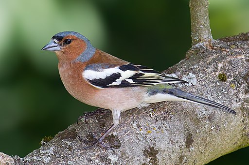
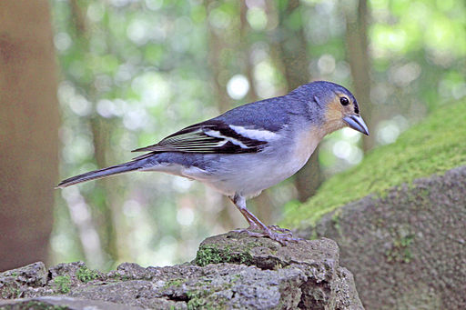
🛝 Make a folder called images and save these two images of the subspecies to it: canariensis.jpg and coelebs.jpg. Then add images of each of the chaffinch subspecies as a multi-panel figure in the introduction

Summary

Quarto is a Mutli-language scientific publishing system for creating dynamic reproducible reports in a many formats. It is based on R Markdown.
The YAML header provides metadata and sets the default behaviour for the document
Code chunk options determine how/whether they run whether code/output is included in the rendered document
Code can be run interactively
“Divs” are used to group content together and apply styling to that content.
Figures, images, tables and equations can be numbered automatically and cross referenced in text. The fig- and tbl- (etc) prefixes are important for this.
You can add citations and references.

Pages made with R (R Core Team 2025), Quarto (Allaire et al. 2024), knitr (Xie 2024, 2015, 2014), kableExtra (Zhu 2024)

References

Allaire, J. J., Charles Teague, Carlos Scheidegger, Yihui Xie, Christophe Dervieux, and Gordon Woodhull. 2024. “Quarto.” https://doi.org/10.5281/zenodo.5960048.

R Core Team. 2025. R: A Language and Environment for Statistical Computing. Vienna, Austria: R Foundation for Statistical Computing. https://www.R-project.org/.

Xie, Yihui. 2014. “Knitr: A Comprehensive Tool for Reproducible Research in R.” In Implementing Reproducible Computational Research, edited by Victoria Stodden, Friedrich Leisch, and Roger D. Peng. Chapman; Hall/CRC.

———. 2015. Dynamic Documents with R and Knitr. 2nd ed. Boca Raton, Florida: Chapman; Hall/CRC. https://yihui.org/knitr/.

———. 2024. Knitr: A General-Purpose Package for Dynamic Report Generation in r. https://yihui.org/knitr/.

Zhu, Hao. 2024. kableExtra: Construct Complex Table with ’Kable’ and Pipe Syntax. https://CRAN.R-project.org/package=kableExtra.

Introduction

Learning Outcomes

Current process

What is Quarto?

Quarto: live demonstration

Key points from the demo

Markdown foundations

Text Formatting

Headings

Header 1

Header 2

Header 3

Header 4

Links & Images

Equations

Divs

Create your own Quarto document

Create a new project

Change some RStudio settings

Your project contains

Edit the YAML header

Add some content

Edit the YAML header: default code chunk options

Adding content

An Introduction

Data import

Data summary

Methods text

Inline code: reproducible reporting

Extract summary information for use in inline code

Figures

Cross referencing figures

Figure legends

A figure legend with a div

Set the figure size and alignment

Two panel figures

The panels

As one figure

Tables

Crossreferencing Tables

Tables - improve format

Tables - improve format

The visual editor!

Citations

Package citations

Citations from DOI

Extra exercises

Summary

References