6 One-way ANOVA revisited

In this chapter we again consider an example with one categorical explanatory variable. However, this time it has more than two groups (or levels). We first use the familiar aov() function to carry out a one-way ANOVA and then use that understanding to help us understand the output of lm(). We will also make predictions from the model and report on our results.

6.1 Introduction to the example

Figure 6.1: Baby Weddell Seals are very cute. By Photo © Samuel Blanc, CC BY-SA 3.0, https://commons.wikimedia.org/w/index.php?curid=3877642

The myoglobin concentration of skeletal muscle (in grams per kilogram of muscle) for three species of seal (see Figure 6.1) is given in seal.txt.

species	myoglobin
Harbour Seal	49.7
Harbour Seal	51.0
Harbour Seal	41.6
Harbour Seal	45.6
Harbour Seal	39.4
Harbour Seal	43.1
Harbour Seal	55.7
Harbour Seal	66.1
Harbour Seal	56.0
Harbour Seal	47.0
Harbour Seal	51.5
Harbour Seal	50.9
Harbour Seal	53.4
Harbour Seal	35.3
Harbour Seal	45.2
Harbour Seal	38.4
Harbour Seal	50.5
Harbour Seal	49.4
Harbour Seal	41.6
Harbour Seal	41.5
Harbour Seal	45.8
Harbour Seal	48.1
Harbour Seal	57.3
Harbour Seal	61.2
Harbour Seal	48.8
Harbour Seal	62.2
Harbour Seal	38.0
Harbour Seal	40.6
Harbour Seal	67.3
Harbour Seal	48.5
Weddell Seal	55.4
Weddell Seal	40.1
Weddell Seal	46.3
Weddell Seal	29.8
Weddell Seal	52.5
Weddell Seal	37.4
Weddell Seal	42.8
Weddell Seal	51.4
Weddell Seal	48.5
Weddell Seal	44.0
Weddell Seal	58.0
Weddell Seal	45.4
Weddell Seal	37.1
Weddell Seal	39.3
Weddell Seal	45.1
Weddell Seal	51.1
Weddell Seal	38.1
Weddell Seal	36.5
Weddell Seal	49.4
Weddell Seal	62.0
Weddell Seal	45.7
Weddell Seal	57.0
Weddell Seal	42.6
Weddell Seal	40.0
Weddell Seal	31.9
Weddell Seal	42.7
Weddell Seal	46.0
Weddell Seal	39.0
Weddell Seal	50.1
Weddell Seal	34.4
Bladdernose Seal	56.2
Bladdernose Seal	48.4
Bladdernose Seal	37.8
Bladdernose Seal	42.8
Bladdernose Seal	27.0
Bladdernose Seal	43.1
Bladdernose Seal	42.4
Bladdernose Seal	29.9
Bladdernose Seal	42.3
Bladdernose Seal	58.1
Bladdernose Seal	32.2
Bladdernose Seal	38.4
Bladdernose Seal	52.6
Bladdernose Seal	53.9
Bladdernose Seal	42.3
Bladdernose Seal	46.4
Bladdernose Seal	44.6
Bladdernose Seal	49.0
Bladdernose Seal	40.2
Bladdernose Seal	41.4
Bladdernose Seal	38.6
Bladdernose Seal	35.1
Bladdernose Seal	48.2
Bladdernose Seal	33.2
Bladdernose Seal	38.4
Bladdernose Seal	26.0
Bladdernose Seal	50.0
Bladdernose Seal	42.6
Bladdernose Seal	47.0
Bladdernose Seal	41.6

The data were collected to determine whether muscle myoglobin differed between species.

There are 2 variables. seal is the explanatory variable; it is categorical with 3 levels, Bladdernose Seal, Harbour Seal and Weddell Seal. myoglobin, a continuous variable, is the response.

We can use the read_delim() function to import the data and visualise it with ggplot().

seal <- read_delim("data-raw/seal.txt", delim = " ")

# create a rough plot of the data  
ggplot(data = seal, aes(x = species, y = myoglobin)) +
  geom_violin()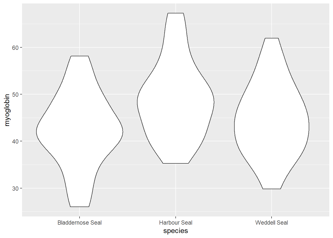

Harbour Seals seem to have higher myoglobin than the other two species and the variance in myoglobin for the three species looks about the same.

Let’s create a summary of the data that will be useful for plotting later:

seal_summary <- seal %>%
  group_by(species) %>%
  summarise(mean = mean(myoglobin),
            std = sd(myoglobin),
            n = length(myoglobin),
            se = std/sqrt(n))

species	mean	std	n	se
Bladdernose Seal	42.3	8.02	30	1.46
Harbour Seal	49.0	8.25	30	1.51
Weddell Seal	44.7	7.85	30	1.43

Our summary confirms that there are thirty individuals of each species and that highest mean is for Harbour Seals and the lowest is for Bladdernose Seals. The variance within each species is similar.

6.2 `aov()` output reminder

The aov() function requires a model formula, myoglobin ~ species, in the familiar format. We also specify the data argument to indicate where the species and myoglobin variables can be found:

mod <- aov(data = seal, myoglobin ~ species)

The output of the summary() function gives us an ANOVA test:

summary(mod)
#             Df Sum Sq Mean Sq F value Pr(>F)   
# species      2    692     346    5.35 0.0064 **
# Residuals   87   5627      65                  
# ---
# Signif. codes:  0 '***' 0.001 '**' 0.01 '*' 0.05 '.' 0.1 ' ' 1

There was a significant difference in myoglobin concentration between seal species (ANOVA: $F$ = 5.352; $d.f.$ = 2, 87; $p$ = 0.006). We need a post-hoc multiple comparison test to discover which pairs of means differ significantly.

6.3 Post-hoc testing for `aov()`

A commonly applied multiple comparison test applied after an significant ANOVA result is the Tukey Honest Significant Difference test:

TukeyHSD(mod)
#   Tukey multiple comparisons of means
#     95% family-wise confidence level
# 
# Fit: aov(formula = myoglobin ~ species, data = seal)
# 
# $species
#                                diff   lwr    upr p adj
# Harbour Seal-Bladdernose Seal  6.69  1.74 11.646 0.005
# Weddell Seal-Bladdernose Seal  2.34 -2.61  7.296 0.499
# Weddell Seal-Harbour Seal     -4.35 -9.30  0.602 0.097

The p-value, adjusted for multiple comparisons is given in the p adj column. In this case, only one of the three pairwise comparisons is significant. Harbour Seals, with the highest myoglobin concentrations ($\bar{x} \pm s.e.$: 49.01 $\pm$ 1.507) ) were significantly higher than Bladdernose Seals with the lowest ($\bar{x} \pm s.e.$: 42.316 $\pm$ 1.464).

The comparisons being made are known as contrasts and this terminology will appear later.

6.4 One-way ANOVAs as linear models

The equation for a one-way ANOVA test is an extension of equation (5.1) for a t-test. It has the same form but additional parameters. If there are three groups, the model is:

\[\begin{equation} E(y_{i})=\beta_{0}+\beta_{1}X1_{i}+\beta_{2}X2_{i} \tag{6.1} \end{equation}\]

The parameter $\beta_{0}$, the intercept, is the value of the response when the categorical explanatory is at its “lowest” level. $X1_{i}$ and $X2_{i}$ are the dummy explanatory variables which take a value of 0 or 1 to toggle on and off the effects of $\beta_{1}$ and $\beta_{2}$ respectively.

$\beta_{1}$ is the difference between the mean of the group represented by the intercept and the next group and $\beta_{2}$ is the difference between the mean of the group represented by the intercept and the group after that.

An additional parameter and dummy variable are added for each additional group so for four groups the equation is:

\[\begin{equation} E(y_{i})=\beta_{0}+\beta_{1}X1_{i}+\beta_{2}X2_{i}+\beta_{3}X3_{i} \tag{6.2} \end{equation}\]

A graphical representation of the terms in a linear model when the explanatory variable is categorical with four groups is given in Figure 6.2.

$A linear model when the explanatory variable is categorical with four groups annotated with the terms used in linear modelling. The measured response values are in pink, the predictions are in green, and the differences between these, known as the residuals, are in blue. The estimated model parameters are indicated: $\beta_{0}$ is the mean of group A; $\beta_{1}$ is what has to be added to $\beta_{0}$ to get the mean of group B; $\beta_{2}$ is what has to be added to $\beta_{0}$ to get the mean of group C; and $\beta_{3}$ is what has to be added to $\beta_{0}$ to get the mean of group D. In this figure, $\beta_{1}$ and $\beta_{2}$ are positive and $\beta_{3}$ is negative. Compare to Figure 2.2.$

Figure 6.2: A linear model when the explanatory variable is categorical with four groups annotated with the terms used in linear modelling. The measured response values are in pink, the predictions are in green, and the differences between these, known as the residuals, are in blue. The estimated model parameters are indicated: $\beta_{0}$ is the mean of group A; $\beta_{1}$ is what has to be added to $\beta_{0}$ to get the mean of group B; $\beta_{2}$ is what has to be added to $\beta_{0}$ to get the mean of group C; and $\beta_{3}$ is what has to be added to $\beta_{0}$ to get the mean of group D. In this figure, $\beta_{1}$ and $\beta_{2}$ are positive and $\beta_{3}$ is negative. Compare to Figure 2.2.

All the $\beta$ values are given relative to $\beta_{0}$. Their sign indicates whether a group mean is bigger (positive) or smaller (negative) than the intercept.

6.5 Applying and interpreting `lm()`

The lm() function is applied to the seal example as follows:

mod <- lm(data = seal, myoglobin ~ species)

Printing mod to the console gives us the estimated model parameters (coefficients):

mod
# 
# Call:
# lm(formula = myoglobin ~ species, data = seal)
# 
# Coefficients:
#         (Intercept)  speciesHarbour Seal  speciesWeddell Seal  
#               42.32                 6.69                 2.34

The equation for the model is: $myoglobin$ = 42.316 + 6.694$speciesHarbour Seal$ + 2.344$speciesWeddell Seal$

The first group of seal is Bladdernose Seal so $\beta_{0}$ is the mean of the Bladdernose seals. $\beta_{1}$ is the coefficient labelled speciesHarbour Seal and means when the variable species takes the value Harbour Seal, $\beta_{1}$ must be added to $\beta_{0}$. The last parameter, $\beta_{2}$, is the coefficient labelled speciesWeddell Seal and means when the variable species takes the value Weddell Seal, $\beta_{2}$ must be added to $\beta_{0}$.

Bladdernose mean is $\beta_{0}$
Harbour mean is $\beta_{0} + \beta_{1}$
Weddell mean is $\beta_{0} + \beta_{2}$

The mean myoglobin in Bladdernose seals is 42.316 kg g^-1, that in Harbour Seals is 42.316 + 6.694 = 49.01 kg g^-1 and in Weddell Seals is 42.316 + 2.344 = 44.66kg g^-1.

More information including statistical tests of the model and its parameters is obtained by using summary():

summary(mod)
# 
# Call:
# lm(formula = myoglobin ~ species, data = seal)
# 
# Residuals:
#     Min      1Q  Median      3Q     Max 
# -16.306  -5.578  -0.036   5.240  18.250 
# 
# Coefficients:
#                     Estimate Std. Error t value            Pr(>|t|)    
# (Intercept)            42.32       1.47   28.82 <0.0000000000000002 ***
# speciesHarbour Seal     6.69       2.08    3.22              0.0018 ** 
# speciesWeddell Seal     2.34       2.08    1.13              0.2620    
# ---
# Signif. codes:  0 '***' 0.001 '**' 0.01 '*' 0.05 '.' 0.1 ' ' 1
# 
# Residual standard error: 8.04 on 87 degrees of freedom
# Multiple R-squared:  0.11,    Adjusted R-squared:  0.0891 
# F-statistic: 5.35 on 2 and 87 DF,  p-value: 0.00643

The Coefficients table gives the estimated $\beta_{0}$, $\beta_{1}$ and $\beta_{2}$ again but along with their standard errors and tests of whether the estimates differ from zero. The estimated mean of the Bladdernose seals is 42.316 $\pm$ 1.468 kg g¹ and this differs significantly from zero ($p$ < 0.001). The estimated difference between the Bladdernose and Harbour seals is 6.694 $\pm$ 2.077 and also differs significantly from zero ($p$ = 0.002). The estimated difference between the Bladdernose and Weddell seals, 2.344 $\pm$ 2.077 kg g¹, does not differ significantly from zero ($p$ = 0.262). The fact that both parameters are positive tells us both of the other two species have higher means than Bladdernose.

The proportion of the variance in the omega which is explained by the model is 0.11 and this is a significant proportion of that variance ($p$ = 0.006).

This is the first time we have a model where the p-value for the model and the p-values for the $\beta$ parameters differ. This is because we are fitting two parameters after the intercept.

Replacing the terms shown in Figure 6.2 with the values in this example gives us 6.3.

$The annotated model with the values from the Seal species example. The measured response values are in pink, the predictions are in green, and the residuals, are in blue. One example of a measured value, a predicted value and the residual is shown for an individual harbour seal. The estimated model parameters are indicated: $\beta_{0}$, the mean of the Bladdernose Seals, is 42.316 kg g1; $\beta_{1}$ is 6.694 thus the mean of Harbour Seals 42.316 + 6.694 = 49.01 kg g^-1; and $\beta_{2}$ is 2.344 thus the mean of Weddell Seals 42.316 + 2.344 = 49.01 kg g^-1. Compare to Figure 6.2.$

Figure 6.3: The annotated model with the values from the Seal species example. The measured response values are in pink, the predictions are in green, and the residuals, are in blue. One example of a measured value, a predicted value and the residual is shown for an individual harbour seal. The estimated model parameters are indicated: $\beta_{0}$, the mean of the Bladdernose Seals, is 42.316 kg g¹; $\beta_{1}$ is 6.694 thus the mean of Harbour Seals 42.316 + 6.694 = 49.01 kg g^-1; and $\beta_{2}$ is 2.344 thus the mean of Weddell Seals 42.316 + 2.344 = 49.01 kg g^-1. Compare to Figure 6.2.

6.6 Getting predictions from the model

We already have the predictions for all possible values of the explanatory variable because it is categorical.

However, the code for using predict is included here, as it was in the last chapter, because it will make it easier to understand more complex examples later. We need to create a dataframe of values for which we want predictions and pass it as an argument to the predict() function.

To create a dataframe with one column of Species values:

predict_for <- data.frame(species = c("Bladdernose Seal",
                                      "Harbour Seal",
                                      "Weddell Seal"))

Remember! The variable and its values have to exactly match those in the model.

The to get the predicted myoglobin content for the three species:

predict_for$pred <- predict(mod, newdata = predict_for)

6.7 Checking assumptions

The two assumptions of the model can be checked using diagnostic plots. The Q-Q plot is obtained with:

plot(mod, which = 2)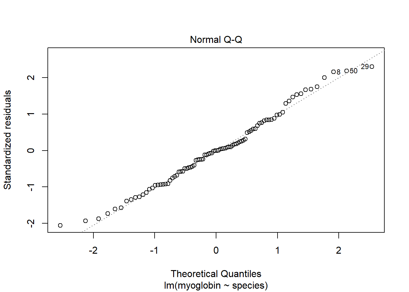

The residual seem to be normally distributed.

Let’s look at the Residuals vs Fitted plot:

plot(mod, which = 1)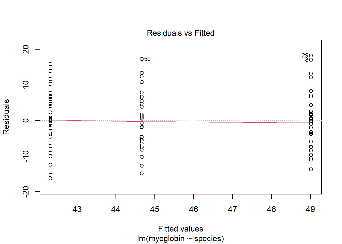

The residuals are equally spread around a horizontal line; the assumptions seem to be met.

6.8 Post-hoc testing for `lm()`

TukeyHSD() requires output from the aov() so we will use the lsmeans() (Least-Squares means) function from the lsmeans package (Lenth 2016) with pairs() from the multcompView package. These two functions can be applied to lm() and glm() outputs.

Load the packages:

library(lsmeans)
library(multcompView)

And run the post-hoc test:

lsmeans(mod, ~ species) %>%
  pairs()
#  contrast                        estimate   SE df t.ratio p.value
#  Bladdernose Seal - Harbour Seal    -6.69 2.08 87  -3.220  0.0050
#  Bladdernose Seal - Weddell Seal    -2.34 2.08 87  -1.130  0.4990
#  Harbour Seal - Weddell Seal         4.35 2.08 87   2.090  0.0970
# 
# P value adjustment: tukey method for comparing a family of 3 estimates

The correction for the multiple testing uses the Tukey method (just like TukeyHSD()).

The results are the same as for using TukeyHSD() as we have done the same tests using a different function.

6.9 Creating a figure

ggplot() +
  geom_jitter(data = seal, 
              aes(x = species, y = myoglobin), 
              width = 0.25, colour = "grey") +
  geom_errorbar(data = seal_summary,
                aes(x = species,
                    ymin = mean,
                    ymax = mean),
                width = .3) +
  geom_errorbar(data = seal_summary,
                aes(x = species,
                    ymin = mean - se,
                    ymax = mean + se),
                width = .5) +
  geom_segment(aes(x = 1, y = 71, xend = 2, yend = 71),
               size = 1) +
  geom_segment(aes(x = 1, y = 71, xend = 1, yend = 69),
               size = 1) +
  geom_segment(aes(x = 2, y = 71, xend = 2, yend = 69),
               size = 1) +
  annotate("text", x = 1.5, y = 73,  label = "**", size = 6) +
  scale_x_discrete(name = "Species") +
  scale_y_continuous(name = expression("Myoglobin concentration g "*Kg^{-1}),
                     expand = c(0, 0),
                     limits = c(0, 75)) +
  theme_classic()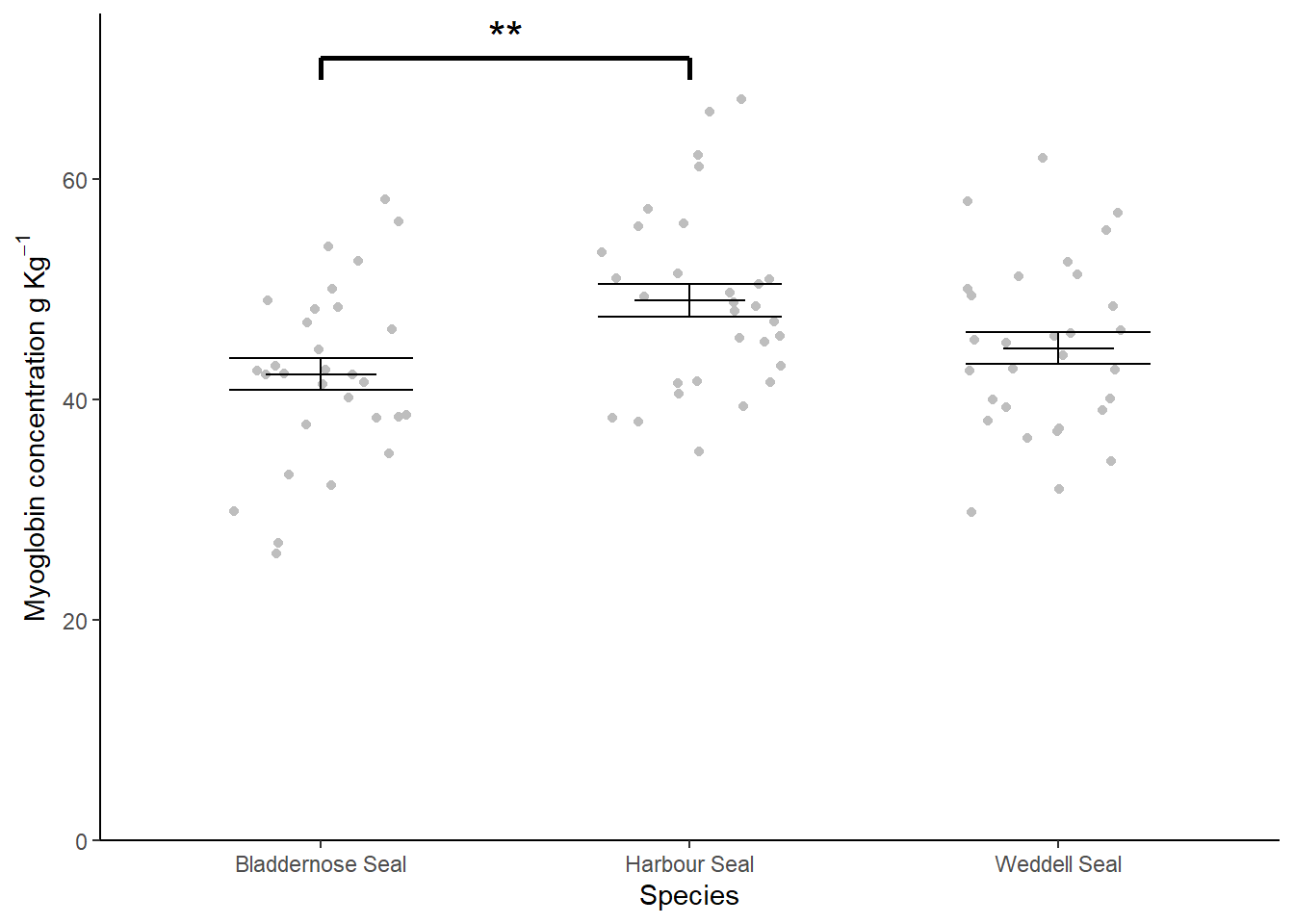

6.10 Reporting the results

There is a significant difference in myoglobin concentration between Seal species (ANOVA: $F$ = 5.352; $d.f.$ = 2, 87; $p$ = 0.006). Post-hoc testing revealed that difference to be between the Harbour Seal with the highest myoglobin concentrations ($\bar{x} \pm s.e.$: 49.01 $\pm$ 1.507) ) and the Bladdernose Seal ($p$ = 0.005) with the lowest ($\bar{x} \pm s.e.$: 42.316 $\pm$ 1.464). See figure 6.4.

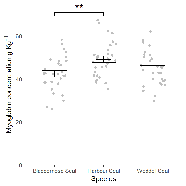
$Muscle myoglobin content of three seal species. Error bars are $\pm 1 S.E.$. ** significant difference at the $p < 0.001$ level.$

Figure 6.4: Muscle myoglobin content of three seal species. Error bars are $\pm 1 S.E.$. ** significant difference at the $p < 0.001$ level.

5 t-tests revisited

7 Two-way ANOVA revisited