2 What are General Linear Models

2.1 Overview

A general linear model describes a continuous response variable as a function of one or more explanatory variables. For a single explanatory variable, the model is:

\[\begin{equation} E(y_{i})=\beta_{0}+\beta_{1}X1_{i} \tag{2.1} \end{equation}\]

Where:

$y$ is the response variable and $X1$ is the explanatory variable.
$i$ is the index of the values so $X1_{i}$ is the $i$th value of $X1$
$E(y_{i})$ is the expected value of $y$ for the $i$th value of $X1$.
$\beta_{0}$ and $\beta_{1}$ are the coefficients - or parameters - in the model. In a single linear regression, $\beta_{0}$ is often called the intercept and $\beta_{1}$ the slope.

The equation (2.1) allows the response, $y$, to be predicted for a given value of the explanatory variable.

Let’s unpack what we mean by $E(y_{i})$, the expected value of $y$. If you measure the response for a particular value of $x$ very many times there would be some distribution of those responses. In the general linear model that distribution is assumed to be normal and its mean is the expected value for $y$, $E(y_{i})$.

Another way of saying that is that in a general linear model, we “model the mean of the response.” That the measured response is drawn from normal distribution with a mean of $E(y_{i})$ is a defining feature of the general linear model.

An additional assumption is that those normal distributions have the same variance for all the $x$ values.

2.2 Model fitting

The process of estimating the model coefficients from your data (set of chosen $X1$ with their measured $y$ values) is known as fitting a linear model. The coefficients are also known as parameters.

The measured response values in your data, $y_{i}$, will differ from the predicted values, $\hat{y}$, randomly and these random differences are known as residuals or errors. Our parameter values are chosen to minimise the sum of the squared residuals. A very commonly used abbreviation for the sum of the squared residuals (or errors) is $SSE$.

\[\begin{equation} SSE = \sum(y_{i}-\hat{y})^2 \tag{2.2} \end{equation}\]

Since the coefficient values are those that minimise the $SSE$, those values are known as least squares estimates. The mean of a sample is also a least squares estimate -

The role played by $SSE$ in estimating our parameters means that it is also used in determining how well our model fits our data. Our model can be considered useful if its predictions are close to the observed data and the smaller the value of $SSE$, the better the fit. In other words, there is little random variance left over in the response. The absolute value of $SSE$ will depend on the size of the $y$ values and the sample size so it would be difficult to compare two models. Instead, we express it as a proportion of the total variation in $y$, $SST$:

\[\begin{equation} SSE / SST \tag{2.3} \end{equation}\]

This is the proportion of variance left over after the model fitting. The proportion of variance explained by the model is a very commonly used metric of model fit and you have probably heard of it - R-squared, $R^2$. It is:

\[\begin{equation} R^2=1-\frac{SSE}{SST} \tag{2.3} \end{equation}\]

If there were no explanatory variables, the value we would predict for the response variable is its mean. Thus a good model should fit the response better than the mean. The output of lm() includes the $R^2$. It represents the proportional improvement in the predictions from the regression model relative to the mean model. It ranges from zero, the model is no better than the mean, to 1, the predictions are perfect. See Figure 2.1.

A linear model with different fits. A) the model is a poor fit - the explanatory variable is no better than the response mean for predicting the response. B) the model is good fit - the explanatory variable explains a high proportion of the variance in the response. C) the model is a perfect fit - the response can be predicted perfectly from the explanatory variable. Measured response values are in pink, the predictions are in green and the dashed blue line gives the mean of the response.

Figure 2.1: A linear model with different fits. A) the model is a poor fit - the explanatory variable is no better than the response mean for predicting the response. B) the model is good fit - the explanatory variable explains a high proportion of the variance in the response. C) the model is a perfect fit - the response can be predicted perfectly from the explanatory variable. Measured response values are in pink, the predictions are in green and the dashed blue line gives the mean of the response.

Since the distribution of the responses for a given $x$ is assumed to be normal and the variances of those distributions are assumed to be homogeneous, both are also true of the residuals. It is our examination of the residuals which allows us to evaluate whether the assumptions are met.

See Figure 2.2 for a graphical representation of linear modelling terms introduced so far. We will reference this figure in later chapters.

$A general linear model annotated with the terms used in modelling. The measured response values are in pink, the predictions are in green, and the differences between these, known as the residuals, are in blue. The estimated model parameters, $\beta_{0}$ (the intercept) and $\beta_{1}$ (the slope) are indicated.$

Figure 2.2: A general linear model annotated with the terms used in modelling. The measured response values are in pink, the predictions are in green, and the differences between these, known as the residuals, are in blue. The estimated model parameters, $\beta_{0}$ (the intercept) and $\beta_{1}$ (the slope) are indicated.

2.3 More than one explanatory variable

When you have more than one explanatory variable these are given as $X2$, $X3$ and so on up to the $p$th explanatory variable. Each explanatory variable has its own $\beta$ coefficient.

The general form of the model is: \[\begin{equation} E(y_{i})=\beta_{0}+\beta_{1}X1_{i}+\beta_{2}X2_{i}+...+\beta_{p}Xp_{i} \tag{2.4} \end{equation}\]

The model has only one intercept which is the value of the response when all the explanatory variables are zero.

There is one problem with $R^2$ as a measure of model fit: the more explanatory variables that are added, the higher the $R^2$. This is true even if the added variables explain a really tiny amount of the variance in the response. Using $R^2$ to select a model would mean always choosing the model with the most variables in it. However, a key aim of statistical modelling is to understand the response and this is easier for simpler models. We want to find a balance between the complexity of the model and its explanatory power. The Adjusted $R^2$ is a way to achieve this. It reduces the $R^2$ for each coefficient added.

A related reason for not including variables that explain only tiny amounts of variance is overfitting. Overfitting occurs when your model fits your data very well but does not generalise. We want models that would predict the response equally well for a new set of data.

2.4 General linear models in R

2.4.1 Building and viewing

T-tests and ANOVA, like regression, can be carried out with the lm() function in R. It uses the same method for specifying the model. When you have one explanatory variable the command is:

lm(data = dataframe, response ~ explanatory)

The response ~ explanatory part is known as the model formula.

When you have two explanatory variable we add the second explanatory variable to the formula using a + or a *. The command is:

lm(data = dataframe, response ~ explanatory1 + explanatory2)

lm(data = dataframe, response ~ explanatory1 * explanatory2)

A model with explanatory1 + explanatory2 considers the effects of the two variables independently. A model with explanatory1 * explanatory2 considers the effects of the two variables and any interaction between them.

We usually assign the output of lm() commands to an object and view it with summary(). The typical workflow would be:

mod <- lm(data = dataframe, response ~ explanatory) summary(mod)

There are two sorts of statistical tests in the output of summary(mod): tests of whether each coefficient is significantly different from zero; and an F-test of the model overall.

The F-test in the last line of the output indicates whether the relationship modelled between the response and the set of explanatory variables is statistically significant.

lm() can be used to perform tests using the General Linear Model including t-tests, ANOVA and regression for response variables which are normally distributed.

Elements of the lm() object include the estimated coefficients, the predicted values and the residuals. These can be accessed with mod$coeffients, mod$fitted.values and mod$residuals respectively.

2.4.2 Getting predictions

mod$fitted.values gives the predicted values for the explanatory variable values actually used in the experiment, i.e., there is a prediction for each row of data. To get predictions for a different set of values we need to make a dataframe of the different set of values and use the predict() function. The typical workflow would be:

predict_for <- data.frame(explanatory = values) predict_for$pred <- predict(mod, newdata = predict_for)

2.4.3 Checking assumptions

The assumptions of the model are checked using the plot() function which produces diagnostic plots to explore the distribution of the residuals. They are not proof of the assumptions being met but allow us to quickly determine if the assumptions are plausible, and if not, how the assumptions are violated and what data points contribute to the violation.

The two plots which are most useful are the “Q-Q” plot (plot 2) and the “Residuals vs Fitted” plot (plot 1). These are given as values to the which argument of plot().

2.4.3.1 The Q-Q plot

The Q-Q plot is a scatterplot of the residuals (standardised to a mean of zero and a standard deviation of 1) against what is expected if the residuals are normally distributed.

plot(mod, which = 2)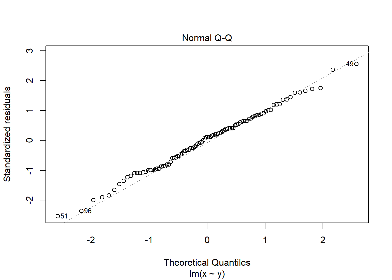

The points should fall roughly on the line if the residuals are normally distributed. In the example above, the residuals appear normally distributed.

The following are two examples in which the residuals are not normally distributed.

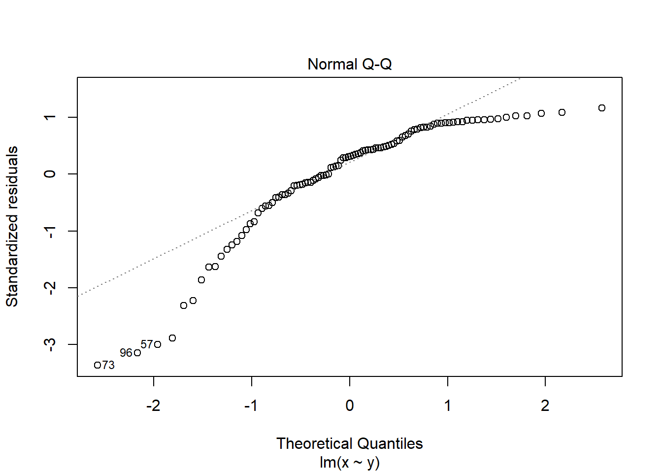
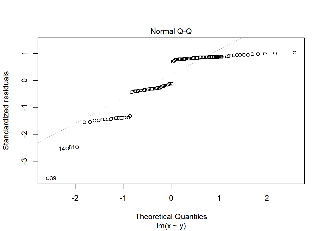
If you see patterns like these you should find an alternative to a general linear model such as a non-parametric test or a generalised linear model. Sometimes, applying a transformation to the response variable will result in better meeting the assumptions.

2.4.3.2 The Residuals vs Fitted plot

The Residuals vs Fitted plot shows if residuals have homogeneous variance or non-linear patterns. Non-linear relationships between explanatory variables and the response will usually show in this plot if the model does not capture the non-linear relationship. For the assumptions to be met, the residuals should be equally spread around a horizontal line as they are here:

plot(mod, which = 1)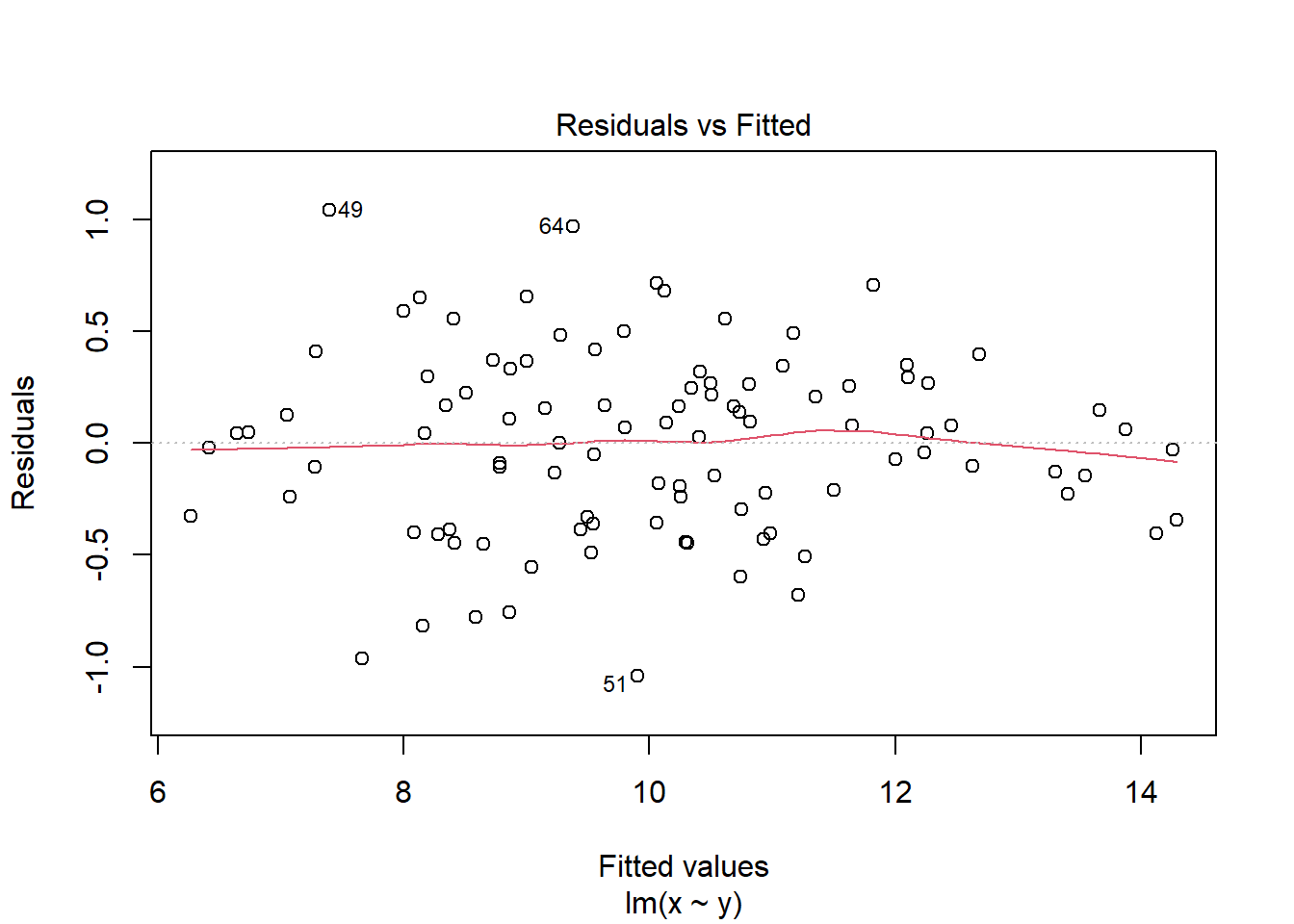

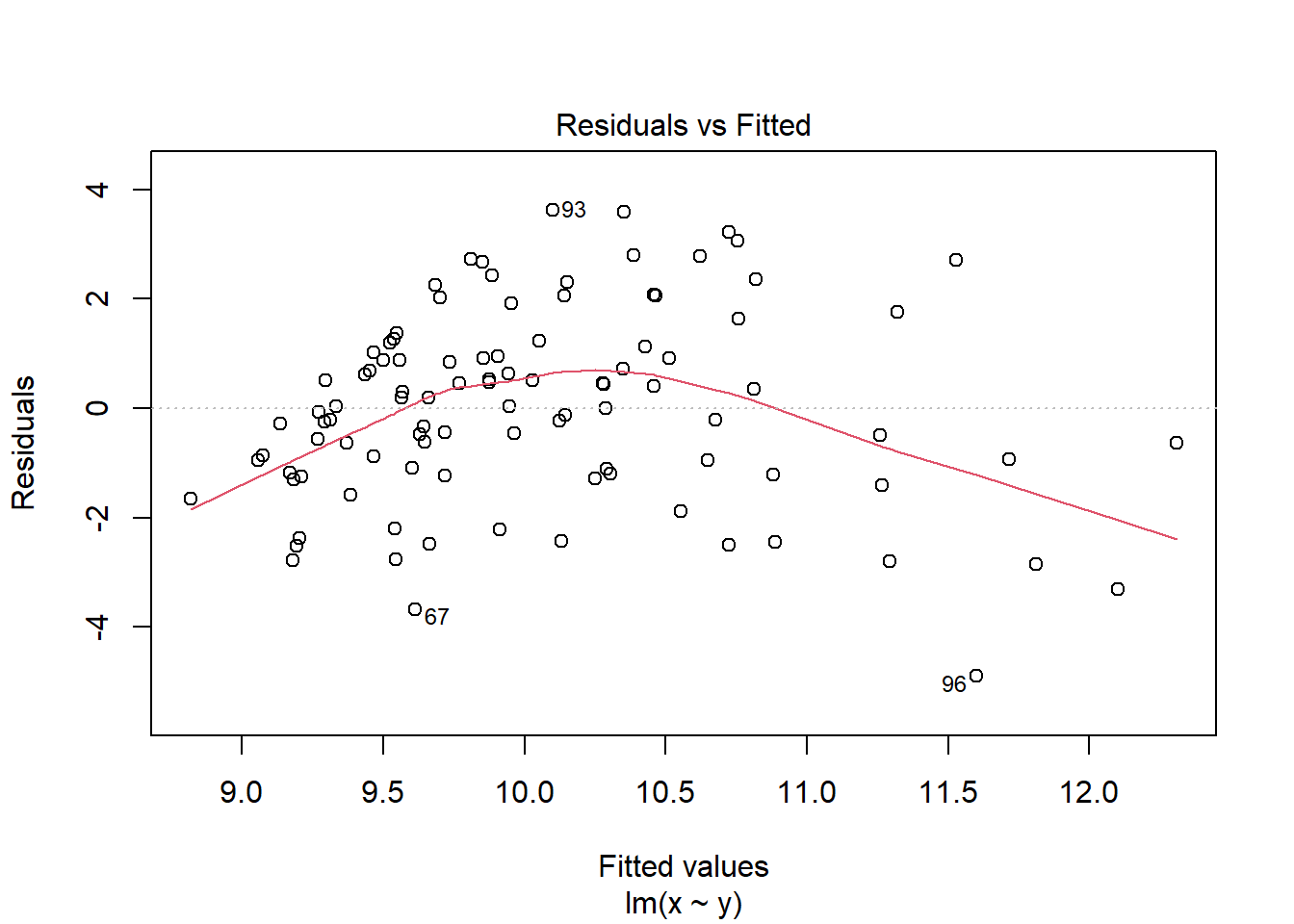
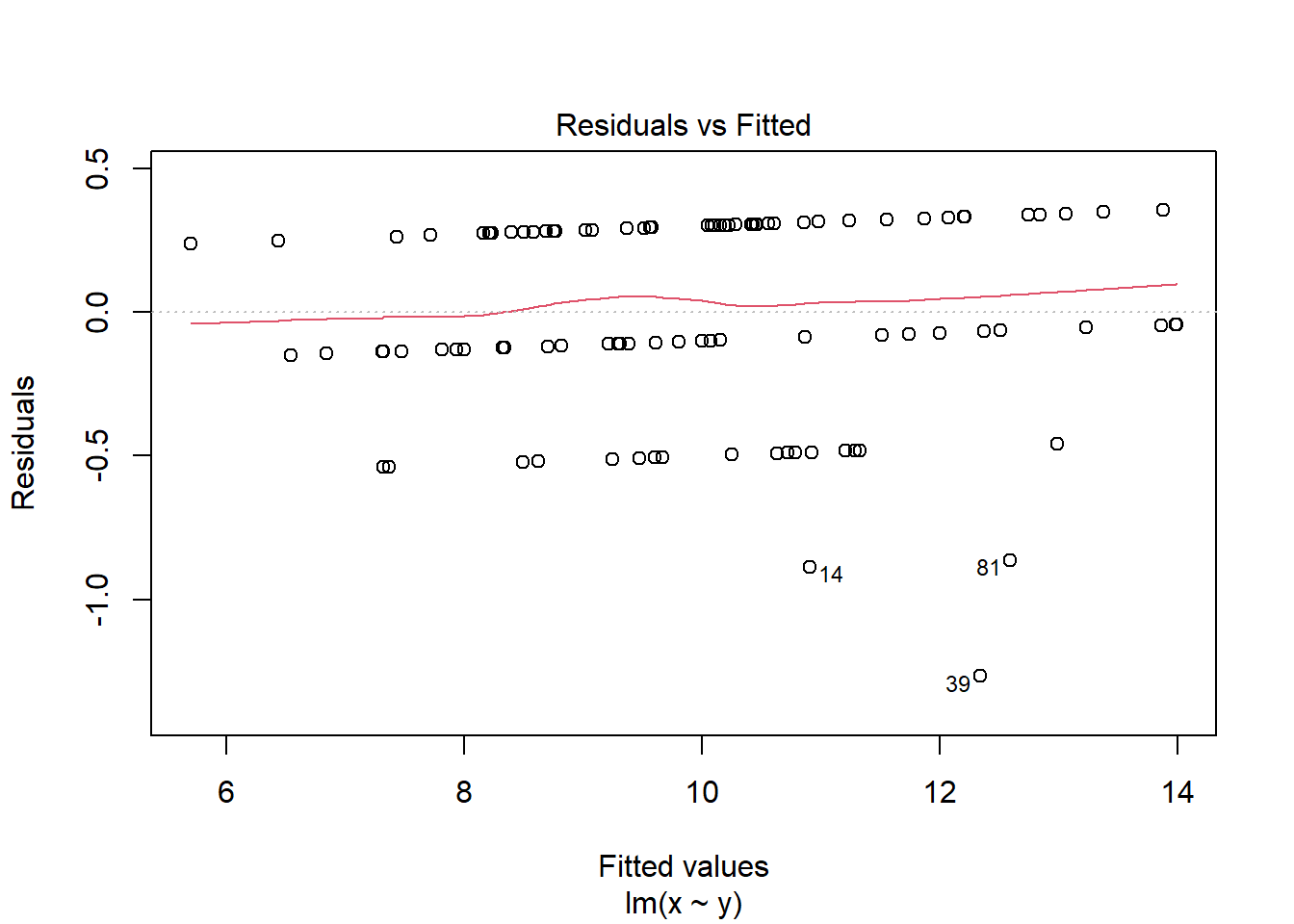
The following are two examples in which the residuals do not have homogeneous variance and display non-linear patterns.

2.5 Reporting

The important information to include when reporting the results of fitting a linear model are the most notable predictions and the significance, direction and magnitude of effects. You need to ensure your reader will understand what the data are saying even if all the numbers and statistical information was removed. For example, that $A$ is much bigger than $B$ or variable $Y$ is influenced by variables $X1$ (a lot) and $X2$ (less so). In relatively simple models, reporting group means or a slope, and statistical test information is enough. In more complex models with many variables is it common to give all the estimated model coefficients in a table.

In addition, your figure should show both the data and the model. This is honest and allows your interpretation to be evaluated.

1 Revision of your Introductory class

3 Terminolgy