7 Two-way ANOVA revisited

In this chapter we turn our attention to designs with two categorical explanatory variables. We will use the same approach that we used in the previous two chapters: first using the familiar aov() function to carry out a two-way ANOVA and then the lm() function. We will also make predictions from the model and report on our results.

7.1 Introduction to the example

Researchers have collected live specimens of two species of periwinkle (see Figure 7.1) from sites in northern England in the Spring and Summer. They take a measure of the gut parasite load by examining a slide of gut contents. The data are in periwinkle.txt.

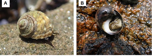
Figure 7.1: Periwinkles are marine gastropod molluscs (slugs and snails). A) Littorina brevicula (PD files - Public Domain, https://commons.wikimedia.org/w/index.php?curid=30577419) B) Littorina littorea. (photographed by Guttorm Flatabø (user:dittaeva). - Photograph taken with an Olympus Camedia C-70 Zoom digital camera. Metainformation edited with Irfanview, possibly cropped with jpegcrop., CC BY-SA 3.0, https://commons.wikimedia.org/w/index.php?curid=324769

para	season	species
58	Spring	Littorina brevicula
51	Spring	Littorina brevicula
54	Spring	Littorina brevicula
39	Spring	Littorina brevicula
65	Spring	Littorina brevicula
67	Spring	Littorina brevicula
60	Spring	Littorina brevicula
54	Spring	Littorina brevicula
47	Spring	Littorina brevicula
66	Spring	Littorina brevicula
51	Spring	Littorina brevicula
43	Spring	Littorina brevicula
62	Spring	Littorina brevicula
55	Spring	Littorina brevicula
58	Spring	Littorina brevicula
43	Spring	Littorina brevicula
69	Spring	Littorina brevicula
71	Spring	Littorina brevicula
64	Spring	Littorina brevicula
58	Spring	Littorina brevicula
51	Spring	Littorina brevicula
70	Spring	Littorina brevicula
55	Spring	Littorina brevicula
47	Spring	Littorina brevicula
54	Spring	Littorina brevicula
43	Spring	Littorina littorea
63	Spring	Littorina littorea
58	Spring	Littorina littorea
61	Spring	Littorina littorea
63	Spring	Littorina littorea
45	Spring	Littorina littorea
45	Spring	Littorina littorea
77	Spring	Littorina littorea
57	Spring	Littorina littorea
49	Spring	Littorina littorea
72	Spring	Littorina littorea
47	Spring	Littorina littorea
78	Spring	Littorina littorea
77	Spring	Littorina littorea
71	Spring	Littorina littorea
69	Spring	Littorina littorea
66	Spring	Littorina littorea
76	Spring	Littorina littorea
75	Spring	Littorina littorea
54	Spring	Littorina littorea
62	Spring	Littorina littorea
58	Spring	Littorina littorea
76	Spring	Littorina littorea
68	Spring	Littorina littorea
84	Spring	Littorina littorea
61	Summer	Littorina brevicula
70	Summer	Littorina brevicula
68	Summer	Littorina brevicula
67	Summer	Littorina brevicula
88	Summer	Littorina brevicula
64	Summer	Littorina brevicula
69	Summer	Littorina brevicula
70	Summer	Littorina brevicula
56	Summer	Littorina brevicula
80	Summer	Littorina brevicula
80	Summer	Littorina brevicula
53	Summer	Littorina brevicula
56	Summer	Littorina brevicula
101	Summer	Littorina brevicula
81	Summer	Littorina brevicula
88	Summer	Littorina brevicula
67	Summer	Littorina brevicula
73	Summer	Littorina brevicula
75	Summer	Littorina brevicula
74	Summer	Littorina brevicula
68	Summer	Littorina brevicula
89	Summer	Littorina brevicula
75	Summer	Littorina brevicula
74	Summer	Littorina brevicula
76	Summer	Littorina brevicula
66	Summer	Littorina littorea
61	Summer	Littorina littorea
51	Summer	Littorina littorea
67	Summer	Littorina littorea
78	Summer	Littorina littorea
79	Summer	Littorina littorea
69	Summer	Littorina littorea
76	Summer	Littorina littorea
86	Summer	Littorina littorea
97	Summer	Littorina littorea
64	Summer	Littorina littorea
68	Summer	Littorina littorea
65	Summer	Littorina littorea
49	Summer	Littorina littorea
62	Summer	Littorina littorea
57	Summer	Littorina littorea
70	Summer	Littorina littorea
62	Summer	Littorina littorea
80	Summer	Littorina littorea
81	Summer	Littorina littorea
85	Summer	Littorina littorea
77	Summer	Littorina littorea
61	Summer	Littorina littorea
59	Summer	Littorina littorea
66	Summer	Littorina littorea

The data were collected to determine whether there was an effect of season or species on parasite load and whether these effects were independent.

There are 3 variables: species and seasonare categorical explanatory variables, each with two levels; para, a continuous variable, is the response.

We can use the read_delim() function to import the data.

periwinkle <- read_delim("data-raw/periwinkle.txt", delim = "\t")

When visualising this data with ggplot() we need to account for both explanatory variables. We can map one to the x-axis and the other to a different aesthetic. Using the fill aesthetic works well for violin plots.

ggplot(data = periwinkle, aes(x = season, y = para, fill = species)) +
  geom_violin()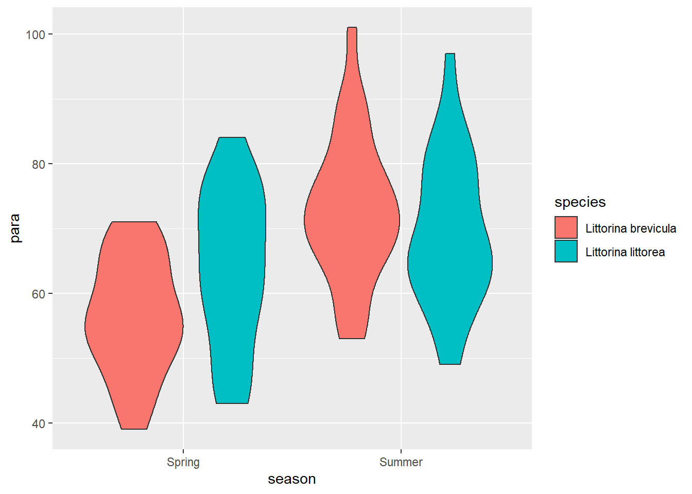

Parasite load seems to be higher for both species in the summer and that effect looks bigger in L.brevicula - it has the lowest spring mean but the highest summer mean.

Let’s create a summary of the data that will be useful for plotting later:

peri_summary <- periwinkle %>% 
  group_by(season, species) %>% 
  summarise(mean = mean(para),
            sd = sd(para),
            n = length(para),
            se = sd / sqrt(n))

season	species	mean	sd	n	se
Spring	Littorina brevicula	56.5	8.88	25	1.78
Spring	Littorina littorea	63.8	11.92	25	2.38
Summer	Littorina brevicula	72.9	11.24	25	2.25
Summer	Littorina littorea	69.4	11.44	25	2.29

The summary confirms both species have a higher mean in the summer and that the difference between the species is reversed - L.brevicula \(-\) L.littorea is -7.28 in the spring but 3.48 in summer.

7.2 aov() output reminder

The aov() function requires a model formula which includes both explanatory variables and the interaction between them in the familiar format: para ~ season * season . We also specify the data argument to indicate where the variables can be found:

mod <- aov(data = periwinkle, para ~ season * species)

The output of the summary() function gives us an ANOVA test:

summary(mod)
#                Df Sum Sq Mean Sq F value   Pr(>F)    
# season          1   3058    3058   25.58 0.000002 ***
# species         1     90      90    0.75    0.387    
# season:species  1    724     724    6.05    0.016 *  
# Residuals      96  11477     120                     
# ---
# Signif. codes:  0 '***' 0.001 '**' 0.01 '*' 0.05 '.' 0.1 ' ' 1

There was a significantly greater number of parasites in the Summer than the Spring (ANOVA: \(F\) = 25.58; \(d.f.\) = 1, 96; \(p\) < 0.001). There was no difference between the species when averaged across the seasons but there was significant interaction (ANOVA: \(F\) = 6.053; \(d.f.\) = 1, 96; \(p\) = 0.016) between season and species with higher numbers infecting L.littorea in the Spring whilst L.brevicula was more heavily parasitized in the Summer.

We need a post-hoc test to discover which comparisons are significant.

7.3 Post-hoc testing for aov

Tukey Honest Significant Difference test is carried out with:

TukeyHSD(mod)
#   Tukey multiple comparisons of means
#     95% family-wise confidence level
# 
# Fit: aov(formula = para ~ season * species, data = periwinkle)
# 
# $season
#               diff  lwr  upr p adj
# Summer-Spring 11.1 6.72 15.4     0
# 
# $species
#                                        diff   lwr  upr p adj
# Littorina littorea-Littorina brevicula  1.9 -2.44 6.24 0.387
# 
# $`season:species`
#                                                        diff     lwr   upr p adj
# Summer:Littorina brevicula-Spring:Littorina brevicula 16.44   8.354 24.53 0.000
# Spring:Littorina littorea-Spring:Littorina brevicula   7.28  -0.806 15.37 0.093
# Summer:Littorina littorea-Spring:Littorina brevicula  12.96   4.874 21.05 0.000
# Spring:Littorina littorea-Summer:Littorina brevicula  -9.16 -17.246 -1.07 0.020
# Summer:Littorina littorea-Summer:Littorina brevicula  -3.48 -11.566  4.61 0.675
# Summer:Littorina littorea-Spring:Littorina littorea    5.68  -2.406 13.77 0.263

The parasite load for L.brevicula increases significantly between spring and summer (\(p\) < 0.001) while that for L.littorea does not. Other significant comparisons are: the spring load of L.brevicula is lower than the summer load of L.littorea (\(p\) < 0.001); and summer load of L.brevicula is higher than the spring load of L.littorea (\(p\) = 0.02).

7.4 Two-way ANOVAs as linear models

The equation for a two-way ANOVA test is an extension of equation (6.1) for a one-way ANOVA test. It has the same form but an additional parameter. If there are two groups in each explanatory variable, the model is:

\[\begin{equation} E(y_{i})=\beta_{0}+\beta_{1}X1_{i}+\beta_{2}X2_{i}+\beta_{3}X1_{i}X2_{i} \tag{6.1} \end{equation}\]

The intercept, \(\beta_{0}\) is the value of the response when both categorical explanatory variables are at their “lowest” level. \(X1_{i}\) is a dummy explanatory variable which indicates the first explanatory variable changing to its second level. It toggles on and off the effects of \(\beta_{1}\). \(X2_{i}\) is a dummy explanatory variable which indicates the second explanatory variable changing to its second level and toggles on and off the effects of \(\beta_{2}\). \(\beta_{3}\) is the interaction effect. If \(X1_{i}\) and \(X2_{i}\) are both 1 \(\beta_{3}\) is the extra effect of that combination above the sum of \(\beta_{1}+\beta_{2}\)

• Spring L.brevicula mean is \(\beta_{0}\)
• Summer L.brevicula mean is \(\beta_{0} + \beta_{1}\)
• Spring L.littorea \(\beta_{0} + \beta_{2}\)
• Summer L.littorea \(\beta_{0} + \beta_{3}\)

The number of parameters in a two-way ANOVA design is: the number of levels in one explanatory \(\times\) the number of levels in the other explanatory. If each explanatory have three levels, there would be nine \(\beta s\)

A graphical representation of the terms in a linear model when there are two explanatory variables each with two groups (or levels) is given in Figure 7.2.

Figure 7.2: A linear model with two explanatory variables each with two levels. ‘Variable 1’ has levels ‘A’ and ‘B’ and ‘Variable 2’ has levels ‘a’ and ‘b.’ Thus there are 2 \(\times\) 2 = 4 groups: Aa, Ab, Ba and Bb. The measured response values are in pink and the predictions are in green. The residuals are not indicated. The estimated model parameters are indicated: \(\beta_{0}\) is the mean of group Aa; \(\beta_{1}\) is what has to be added to \(\beta_{0}\) to get the mean of group Ab; \(\beta_{2}\) is what has to be added to \(\beta_{0}\) to get the mean of group Ba; and \(\beta_{3}\) is what has to be added to \(\beta_{0}\) in addition to \(\beta_{1}\) and \(\beta_{2}\) to get the mean of group Bb. In this figure, all parameters are positive. Compare to Figure 2.2.

The intercept, \(\beta_{0}\)is the response when both explanatory variable is at their first group and all the other \(\beta s\) are given relative to this.

The interaction parameters give the effect of the combination in addition to the sum of their independent effects

7.5 Applying and interpreting lm()

The lm() function is applied to the periwinkle example as follows:

mod <- lm(data = periwinkle, para ~ season * species)

Printing mod to the console gives us the estimated model parameters (coefficients):

mod
# 
# Call:
# lm(formula = para ~ season * species, data = periwinkle)
# 
# Coefficients:
#                            (Intercept)                            seasonSummer  
#                                  56.48                                   16.44  
#              speciesLittorina littorea  seasonSummer:speciesLittorina littorea  
#                                   7.28                                  -10.76

The equation for the model is: \(para\) = 56.48 + 16.44\(speciesLittorina littorea\) + 7.28\(seasonSummer:speciesLittorina littorea\)

The first group of season is Spring and the first group of species is Littorina breviculaso \(\beta_{0}\) is the mean of L.brevicula in the spring, 56.48.

\(\beta_{1}\) is the coefficient labelled seasonSummer and means when the variable season takes the value Summer, \(\beta_{1}\) must be added to \(\beta_{0}\) - the mean of L.brevicula in the summer is \(\beta_{0}+\beta_{1}\) = 56.48 \(+\) 16.44 \(=\) 72.92.
The coefficient labelled speciesLittorina littorea is \(\beta_{2}\). When species becomes Littorina littorea, \(\beta_{1}\) must be added to \(\beta_{0}\) thus the mean of L.littorea in spring is \(\beta_{0}+\beta_{2}\) = 56.48 \(+\) 7.28 \(=\) 63.76.

If both season becomes Summer and species becomes Littorina littorea you would expect the effect to be \(\beta_{0}+\beta_{1}+\beta_{2}\). The coefficient labelled seasonSummer:speciesLittorina littorea, \(\beta_{3}\) is the effect that is additional to that sum. An interaction occurs when the combined effect of two variables differs from just adding the independent effects. The mean of L.littorea in summer is \(\beta_{0}+\beta_{1}+\beta_{2}+\beta_{3}\) = 56.48 \(+\) 16.44 \(+\) 7.28 \(+\) -10.76 \(=\) 69.44.

More information including statistical tests of the model and its parameters is obtained by using summary():

summary(mod)
# 
# Call:
# lm(formula = para ~ season * species, data = periwinkle)
# 
# Residuals:
#    Min     1Q Median     3Q    Max 
# -20.76  -6.13  -1.10   8.12  28.08 
# 
# Coefficients:
#                                        Estimate Std. Error t value
# (Intercept)                               56.48       2.19   25.83
# seasonSummer                              16.44       3.09    5.32
# speciesLittorina littorea                  7.28       3.09    2.35
# seasonSummer:speciesLittorina littorea   -10.76       4.37   -2.46
#                                                    Pr(>|t|)    
# (Intercept)                            < 0.0000000000000002 ***
# seasonSummer                                     0.00000069 ***
# speciesLittorina littorea                             0.021 *  
# seasonSummer:speciesLittorina littorea                0.016 *  
# ---
# Signif. codes:  0 '***' 0.001 '**' 0.01 '*' 0.05 '.' 0.1 ' ' 1
# 
# Residual standard error: 10.9 on 96 degrees of freedom
# Multiple R-squared:  0.252,   Adjusted R-squared:  0.229 
# F-statistic: 10.8 on 3 and 96 DF,  p-value: 0.00000355

The Coefficients table gives the estimated \(\beta_{0}\), \(\beta_{1}\), \(\beta_{2}\) and \(\beta_{3}\) again but along with their standard errors and tests of whether the estimates differ from zero.

The estimated mean of L.brevicula in the spring is 56.48 \(\pm\) 2.187 and this differs significantly from zero (\(p\) < 0.001). The estimated difference between L.brevicula in the spring and L.brevicula in the summer is 16.44 \(\pm\) 3.093 and also differs significantly from zero (\(p\) < 0.001).

The estimated difference between L.brevicula in the spring and L.littorea in the spring, 7.28 \(\pm\) 3.093 differs significantly from zero (\(p\) = 0.021).

The proportion of the variance in parasite load explained by the model is 0.252 and this is a significant proportion of that variance (\(p\) < 0.001).

We are fitting three parameters in addition to the intercept which means the p-value for the model, and the p-values for the \(\beta\) parameters, differ. This was also true for one-way ANOVA.

Replacing the terms shown in Figure 7.2 with the values in this example gives us 7.3.

Figure 7.3: The annotated model with the values from the parasite load of preiwinkle example. The measured response values are in pink and the predictions are in green. The estimated model parameters are indicated: \(\beta_{0}\), the mean of L.brevicula in the spring, is 56.48; \(\beta_{1}\) is 16.44 thus the mean of L.brevicula in the summer 56.48 + 16.44 = 72.92; \(\beta_{2}\) is 7.28 thus the mean of L.littorea in the spring 56.48 + 7.28 = 72.92; and the L.littorea in the summer is \(\beta_{0}+\beta_{1}+\beta_{2}+\beta_{3}\) = 56.48 \(+\) 16.44 \(+\) 7.28 \(+\) -10.76 \(=\) 69.44. Compare to Figure 7.2.

7.6 Getting predictions from the model

We already have the predictions for all possible combinations of values of the explanatory variables because both are categorical.

However, the code for using predict is included here, as it was in the previous two chapters chapter, because it will make it easier to understand more complex examples later. We need to create a dataframe of values for which we want predictions and pass it as an argument to the predict() function.

To create a dataframe with one column of species values and one column of season values:

predict_for <- data.frame(species = rep(c("Littorina brevicula", "Littorina littorea"), each = 2),
                          season = rep(c("Spring", "Summer"), times = 2))

Remember! The variable and its values have to exactly match those in the model.

species	season
Littorina brevicula	Spring
Littorina brevicula	Summer
Littorina littorea	Spring
Littorina littorea	Summer

Then, to get the predicted parasite load for each of the four groups:

predict_for$pred <- predict(mod, newdata = predict_for)

species	season	pred
Littorina brevicula	Spring	56.5
Littorina brevicula	Summer	72.9
Littorina littorea	Spring	63.8
Littorina littorea	Summer	69.4

7.7 Checking assumptions

The two assumptions of the model can be checked using diagnostic plots. The Q-Q plot is obtained with:

plot(mod, which = 2)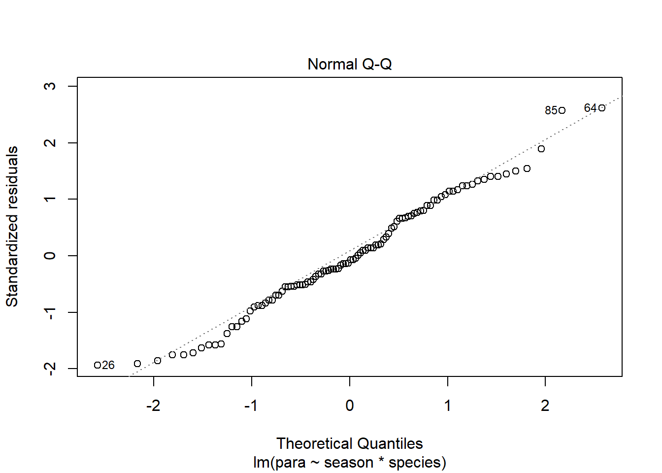

The residual seem to be normally distributed.

Let’s look at the Residuals vs Fitted plot:

plot(mod, which = 1)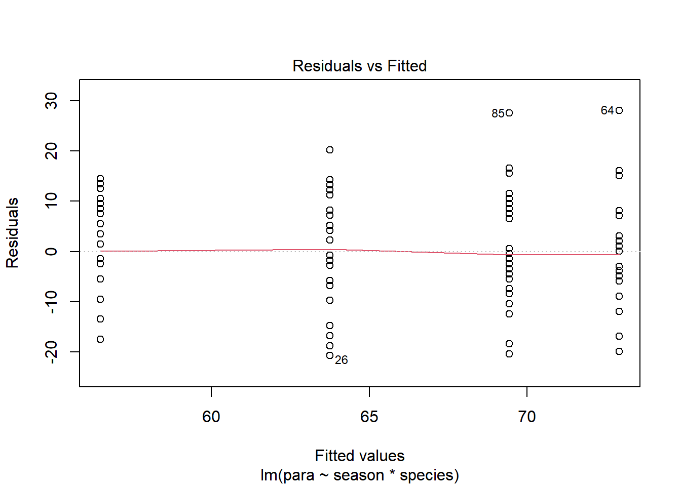

The residuals are equally spread around a horizontal line; the assumptions seem to be met.

7.8 Post-hoc testing for lm()

TukeyHSD() requires output from the aov() so we will use the lsmeans() (Least-Squares means) function from the lsmeans package (Lenth 2016) with pairs() from the multcompView package. These two functions can be applied to lm() and glm() outputs.

Load the packages:

library(lsmeans)
library(multcompView)

And run the post-hoc test:

lsmeans(mod, ~ species) %>%
  pairs()
#  contrast                                 estimate   SE df t.ratio p.value
#  Littorina brevicula - Littorina littorea     -1.9 2.19 96  -0.869  0.3870
# 
# Results are averaged over the levels of: season

The correction for the multiple testing uses the Tukey method (just like TukeyHSD()).

The results are the same as for using TukeyHSD() as we have done the same tests using a different function.

7.9 Creating a figure

# palette
# blue, pink, green triadic
pal4 <- c("#256c7a", "#7a256c", "#6c7a25")

ggplot() +
  geom_point(data = periwinkle, aes(x = season,
                                    y = para,
                                    colour = species),
             position = position_jitterdodge(dodge.width = 1,
                                             jitter.width = 0.4,
                                             jitter.height = 0),
             size = 2) +
  geom_errorbar(data = peri_summary, 
                aes(x = season, ymin = mean - se, ymax = mean + se, group = species),
                width = 0.4, size = 1,
                position = position_dodge(width = 1)) +
  geom_errorbar(data = peri_summary, 
                aes(x = season, ymin = mean, ymax = mean, group = species),
                width = 0.3, size = 1,
                position = position_dodge(width = 1) ) +
  scale_x_discrete(name = "Season") +
  scale_y_continuous(name = "Number of parasites",
                     expand = c(0, 0),
                     limits = c(0, 128)) +
  scale_colour_manual(values = pal4[1:2],
                      labels = c(bquote(italic("L.brevicula")),
                                 bquote(italic("L.littorea")))) +
  # Spring:Littorina brevicula-Summer:Littorina littorea *
  annotate("segment", 
           x = 1.25, xend = 1.75, 
           y = 110, yend = 110,
           colour = "black") +
  annotate("segment", 
           x = 1.25, xend = 1.25,
           y = 110, yend = 105,
           colour = "black") +
  annotate("segment", 
           x = 1.75, xend = 1.75,
           y = 110, yend = 105,
           colour = "black") +
  annotate("text", 
           x = 1.5,  y = 112,
           label = "***", size = 6) +
  # Summer:Littorina brevicula-Spring:Littorina littorea: ***
  annotate("segment", 
           x = 1.25, xend = 0.75,
           y = 90, yend = 90,
           colour = "black") +
  annotate("segment", 
           x = 1.25, xend = 1.25,
           y = 90, yend = 85,
           colour = "black") +
  annotate("segment", 
           x = 0.75, xend = 0.75,
           y = 90, yend = 85,
           colour = "black") +
  annotate("text", x = 1,  y = 92,
           label = "*", size = 6) +
# Summer:Littorina littorea-Spring:Littorina littorea: ***
  annotate("segment",
           x = 0.75, xend = 1.75,
           y = 120, yend = 120,
           colour = "black") +
  annotate("segment",
           x = 0.75, xend = 0.75,
           y = 120, yend = 115,
           colour = "black") +
  annotate("segment",
           x = 1.75, xend = 1.75,
           y = 120, yend = 115,
           colour = "black") +
  annotate("text", x = 1.25,  y = 123,
           label = "***", size = 6) +
  theme_classic() +
  theme(legend.title = element_blank(),
        legend.position = c(0.85, 0.98))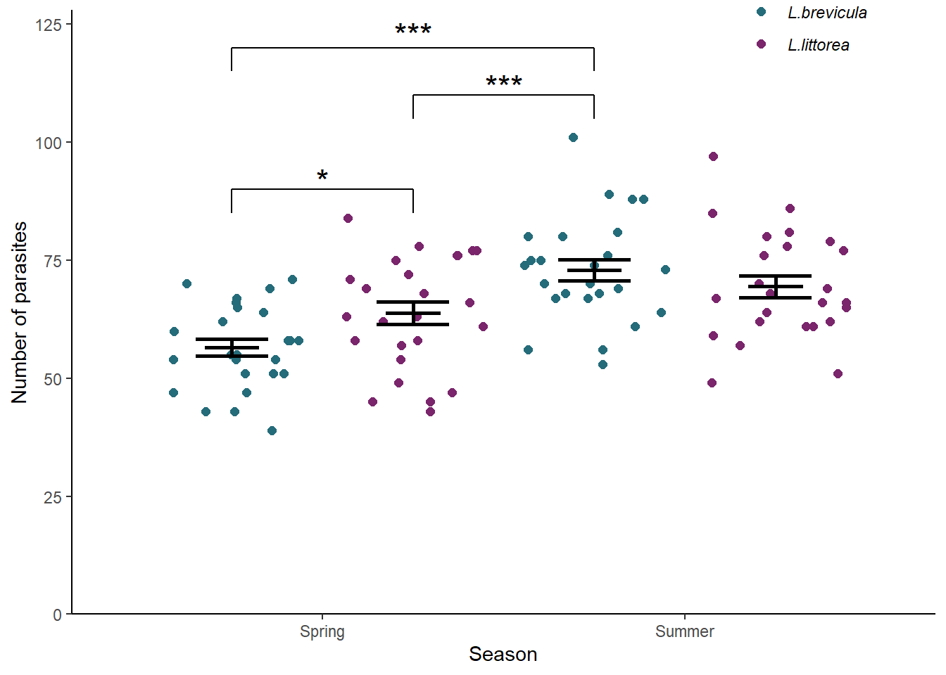 

7.10 Reporting the results

to add

See figure 7.4.

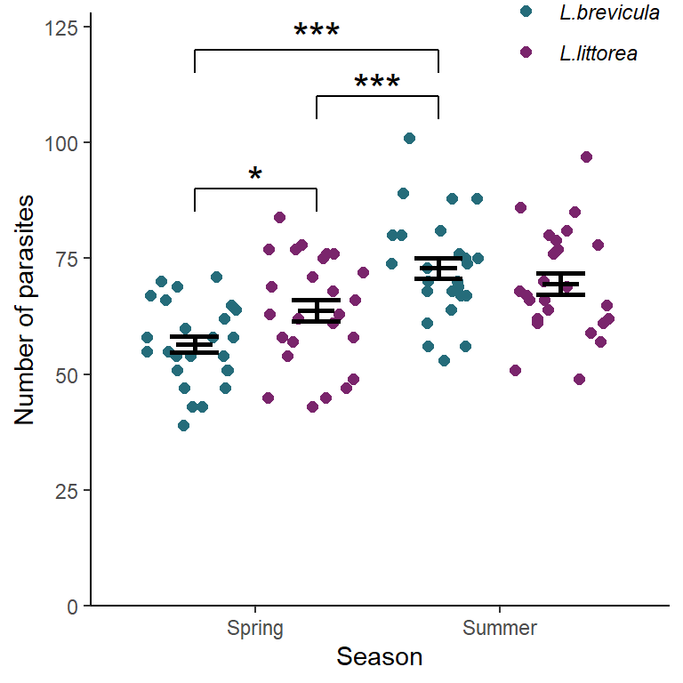
Figure 7.4: The effect of season on the parasite load of two species of periwinkle. Error bars are \(\pm 1 S.E.\). *** significant difference at the \(p < 0.001\) level, ** at the \(p < 0.01\) level and * the \(p < 0.05\) level.