Workflow for VFA analysis
Kelly’s project
Introduction
I have some data and information from Kelly. I have interpreted it and written some code to do the calculations.
However, Kelly hasn’t had a chance to look at it yet so I am providing the exact information and data he supplied along with my suggested workflow based on my interpretation of the data and info.
Exact information supplied by Kelly
The file is a CSV file, with some notes on top and the data in the following order, post notes and headers. Please note that all chemical data is in millimolar. There are 62 rows of actual data.
Sample Name – Replicate, Time (days), Acetate, Propanoate, Isobutyrate, Butyrate, Isopentanoate, Pentanoate, Isohexanoate, Hexanoate
The students should be able to transform the data from mM to mg/L, and to g/L. To do this they only need to multiply the molecular weight of the compound (listed in the notes in the file) by the concentration in mM to get mg/L. Obviously to get g/L they will just divide by 1000. They should be able to graph the VFA concentrations with time.
They should also be able to do a simple flux measurement, which is the change in VFA concentration over a period of time, divided by weight or volume of material. In this case it might be equal to == Delta(Acetate at 3 days - Acetate at 1 day)/Delta (3days - 1day)/50 mls sludge. This would provide a final flux with the units of mg acetate per ml sludge per day. Let me know if this isn’t clear.
Perhaps more importantly they should be able to graph and extract the reaction rate, assuming a first order chemical/biological reaction and an exponential falloff rate. I found this as a starting point (https://martinlab.chem.umass.edu/r-fitting-data/) , but I assume Emma has something much more effective already in the pipeline.
Emma’s Worklflow interpretation
I created these two data files from the original.
- 8 VFA in mM for 60 samples vfa.csv. There were 63 rows of data in the original file. There were no time 0 for one treatment and all values were zero for the other treatment so I removed those.
- Two treatments: straw (CN10) and water (NC)
- 10 time points: 1, 3, 5, 9, 11, 13, 16, 18, 20, 22
- three replicates per treatment per time point
- 2 x 10 x 3 = 60 groups
- 8 VFA with concentration in mM (millimolar): acetate, propanoate, isobutyrate, butyrate, isopentanoate, pentanoate, isohexanoate, hexanoate
- Molecular weights for each VFA in grams per mole mol_wt.txt VFAs from AD vials
We need to:
- Calculate Change in VFA g/l with time
- Recalculate the data into grams per litre - convert to molar: 1 millimolar to molar = 0.001 molar - multiply by the molecular weight of each VFA
- Calculate the percent representation of each VFA, by mM and by weight
- Calculate the flux (change in VFA concentration over a period of time, divided by weight or volume of material) of each VFA, by mM and by weight
- Graph and extract the reaction rate, assuming a first order chemical/biological reaction and an exponential falloff rate
Getting started
🎬 Start RStudio from the Start menu
🎬 Make an RStudio project. Be deliberate about where you create it so that it is a good place for you
🎬 Use the Files pane to make new folders for the data. I suggest data-raw and data-processed
🎬 Make a new script called analysis.R to carry out the rest of the work.
🎬 Load tidyverse (Wickham et al. 2019) for importing, summarising, plotting and filtering.
Examine the data
🎬 Save the files to data-raw. Open them and examine them. You may want to use Excel for the csv file.
🎬 Answer the following questions:
- What is in the rows and columns of each file?
- How many rows and columns are there in each file?
- How are the data organised ?
Import
🎬 Import
vfa_cummul <- read_csv("data-raw/vfa.csv") |> janitor::clean_names()🎬 Split treatment and replicate to separate columns so there is a treatment column:
📢 This code depends on the sample_replicate column being in the form treatment-replicate. In the sample data CN10 and NC are the treatments. The replicate is a number from 1 to 3. The value does include a encoding for time. You might want to edit your file to match this format.
The provided data is cumulative/absolute. We need to calculate the change in VFA with time. There is a function, lag() that will help us do this. It will take the previous value and subtract it from the current value. We need to do that separately for each sample_replicate so we need to group by sample_replicate first. We also need to make sure the data is in the right order so we will arrange by sample_replicate and time_day.
1. Calculate Change in VFA g/l with time
🎬 Create dataframe for the change in VFA 📢 and the change in time
vfa_delta <- vfa_cummul |>
    group_by(sample_replicate)  |>
    arrange(sample_replicate, time_day) |>
    mutate(acetate = acetate - lag(acetate),
           propanoate = propanoate - lag(propanoate),
           isobutyrate = isobutyrate - lag(isobutyrate),
           butyrate = butyrate - lag(butyrate),
           isopentanoate = isopentanoate - lag(isopentanoate),
           pentanoate = pentanoate - lag(pentanoate),
           isohexanoate = isohexanoate - lag(isohexanoate),
           hexanoate = hexanoate - lag(hexanoate),
           delta_time = time_day - lag(time_day))
Now we have two dataframes, one for the cumulative data and one for the change in VFA and time. Note that the VFA values have been replaced by the change in VFA but the change in time is in a separate column. I have done this because we later want to plot flux (not yet added) against time
📢 This code also depends on the sample_replicate column being in the form treatment-replicate. lag is calculating the difference between a value at one time point and the next for a treatment-replicate combination.
2. Recalculate the data into grams per litre
To make conversions from mM to g/l we need to do mM * 0.001 * MW. We will import the molecular weight data, pivot the VFA data to long format and join the molecular weight data to the VFA data. Then we can calculate the g/l. We will do this for both the cumulative and delta dataframes.
🎬 import molecular weight data
mol_wt <- read_table("data-raw/mol_wt.txt") |>
  mutate(vfa = tolower(vfa))
🎬 Pivot the cumulative data to long format:
vfa_cummul <- vfa_cummul |>
  pivot_longer(cols = -c(sample_replicate,
                         treatment,
                         replicate,
                         time_day),
               values_to = "conc_mM",
               names_to = "vfa")
View vfa_cummul to check you understand what you have done.
🎬 Join molecular weight to data and calculate g/l (mutate to convert to g/l * 0.001 * MW):
View vfa_cummul to check you understand what you have done.
Repeat for the delta data.
🎬 Pivot the change data, delta_vfa to long format (📢 delta_time is added to the list of columns that do not need to be pivoted but repeated):
vfa_delta <- vfa_delta |>
  pivot_longer(cols = -c(sample_replicate,
                         treatment,
                         replicate,
                         time_day,
                         delta_time),
               values_to = "conc_mM",
               names_to = "vfa")
View vfa_delta to check it looks like vfa_cummul
🎬 Join molecular weight to data and calculate g/l (mutate to convert to g/l * 0.001 * MW):
3. Calculate the percent representation of each VFA
by mM and by weight
🎬 Add a column which is the percent representation of each VFA for mM and g/l:
Graphs for info so far
🎬 Make summary data for graphing
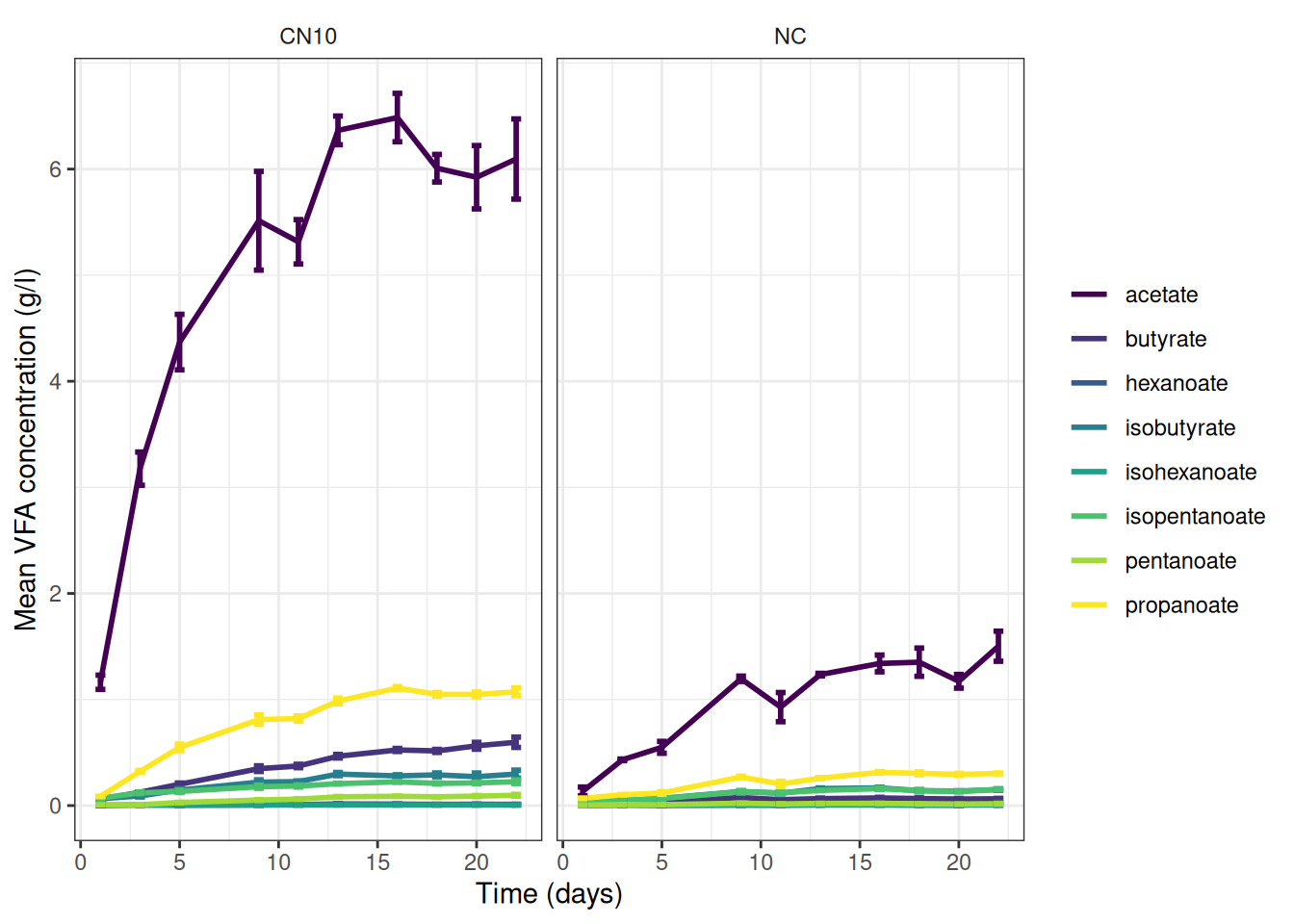
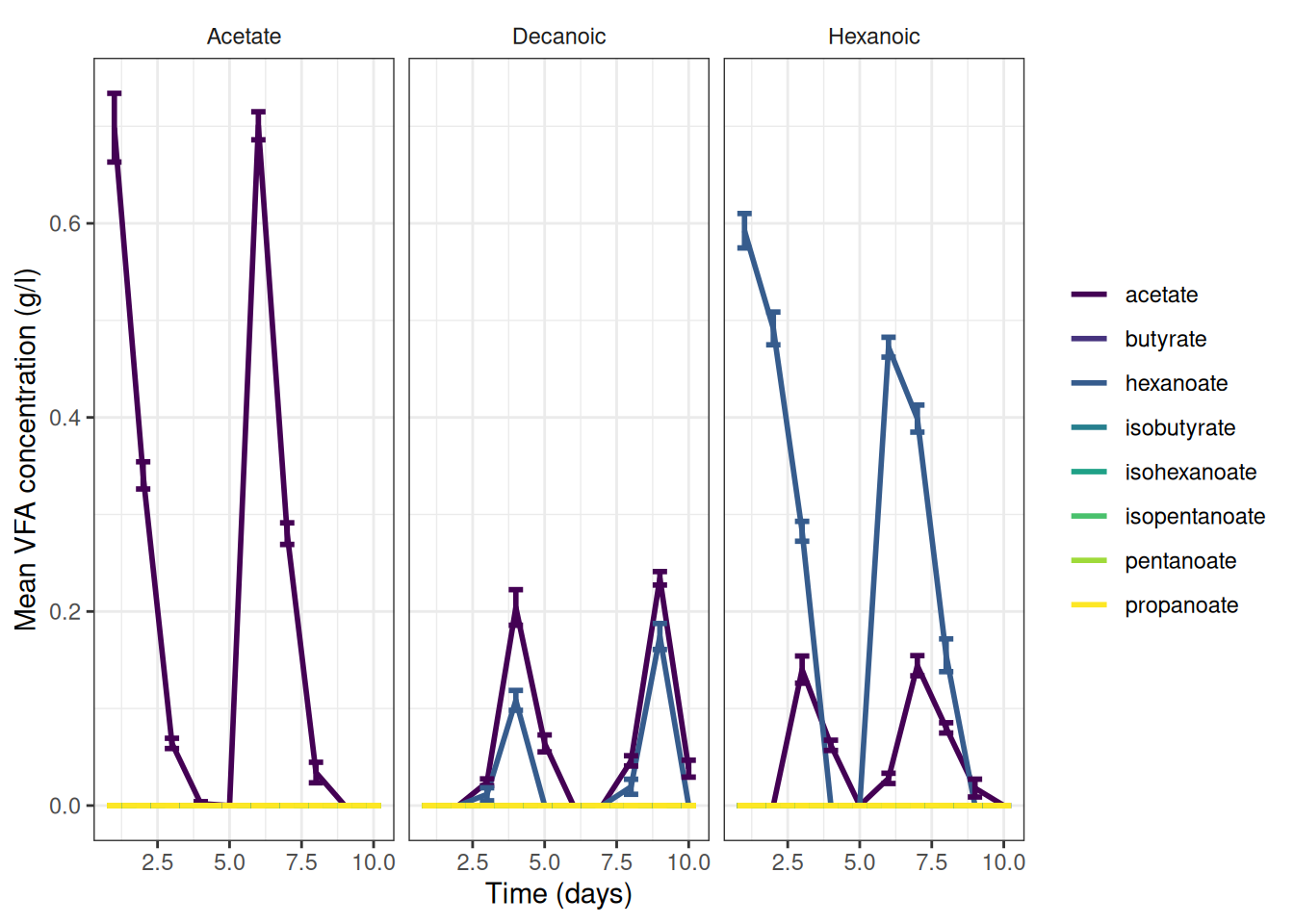
🎬 Graph the cumulative data, grams per litre:
vfa_cummul_summary |>
  ggplot(aes(x = time_day, colour = vfa)) +
  geom_line(aes(y = mean_g_l),
            linewidth = 1) +
  geom_errorbar(aes(ymin = mean_g_l - se_g_l,
                    ymax = mean_g_l + se_g_l),
                width = 0.5,
                show.legend = F,
                linewidth = 1) +
  scale_color_viridis_d(name = NULL) +
  scale_x_continuous(name = "Time (days)") +
  scale_y_continuous(name = "Mean VFA concentration (g/l)") +
  theme_bw() +
  facet_wrap(~treatment) +
  theme(strip.background = element_blank())
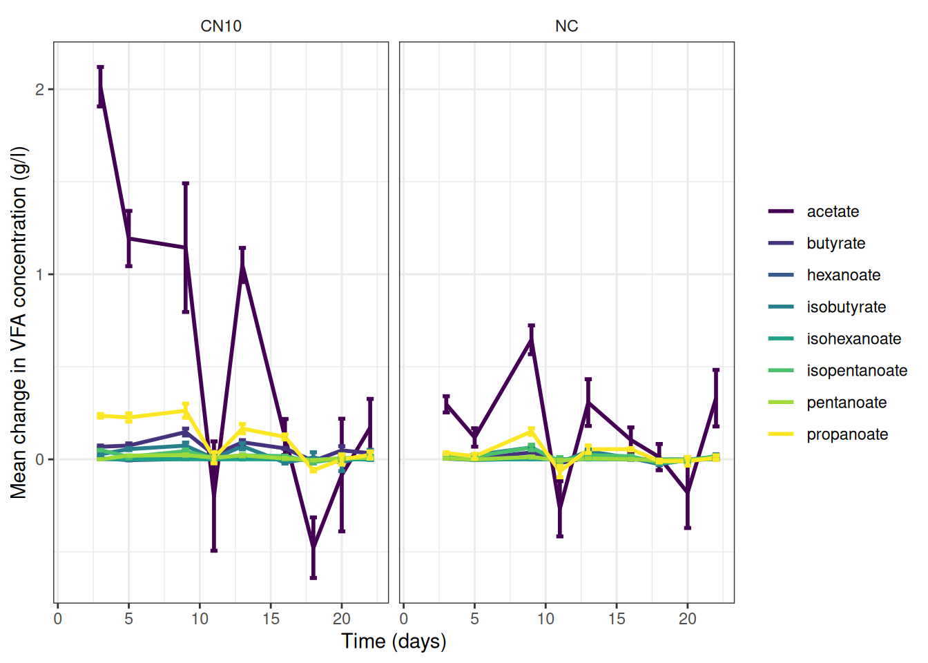
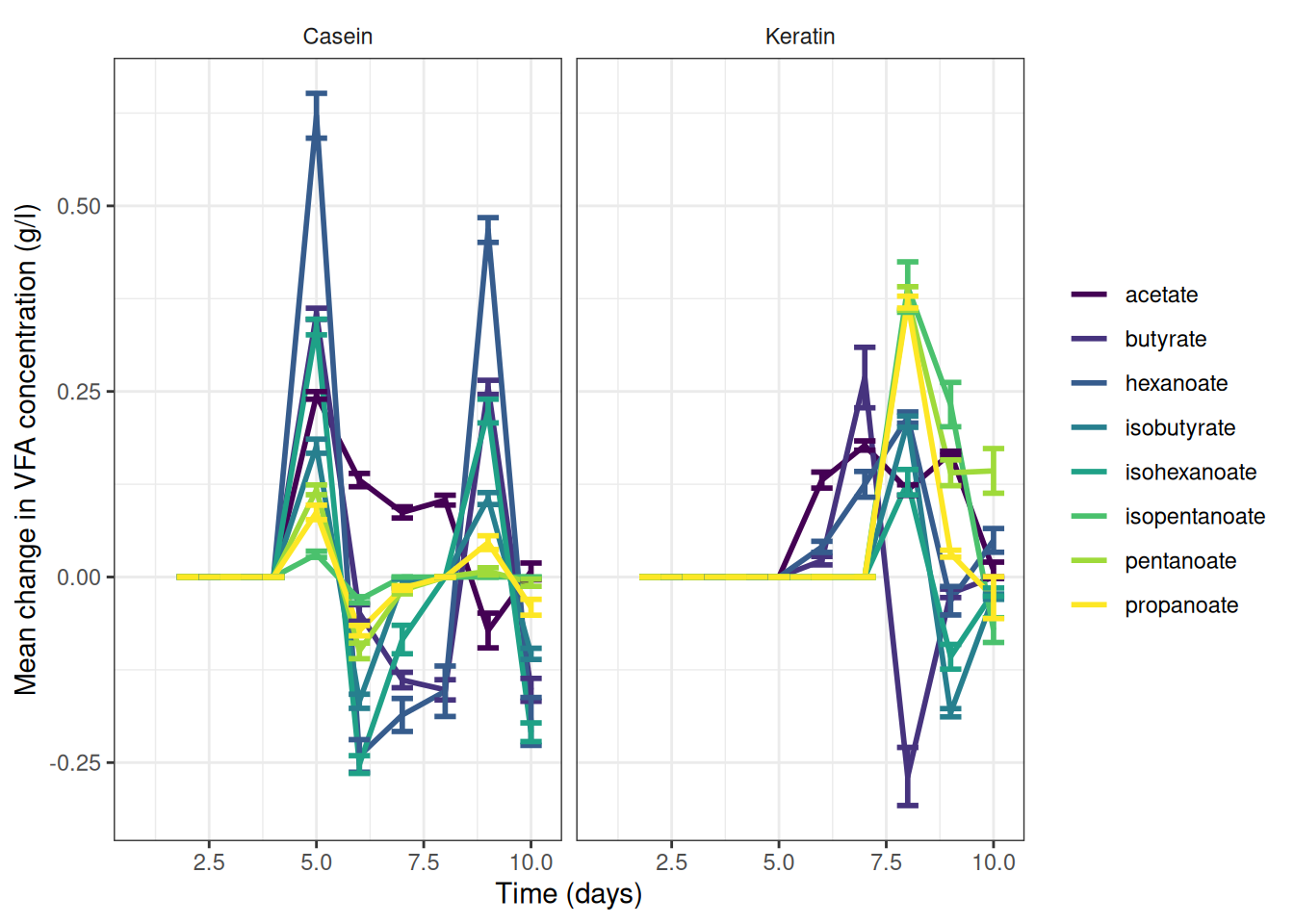
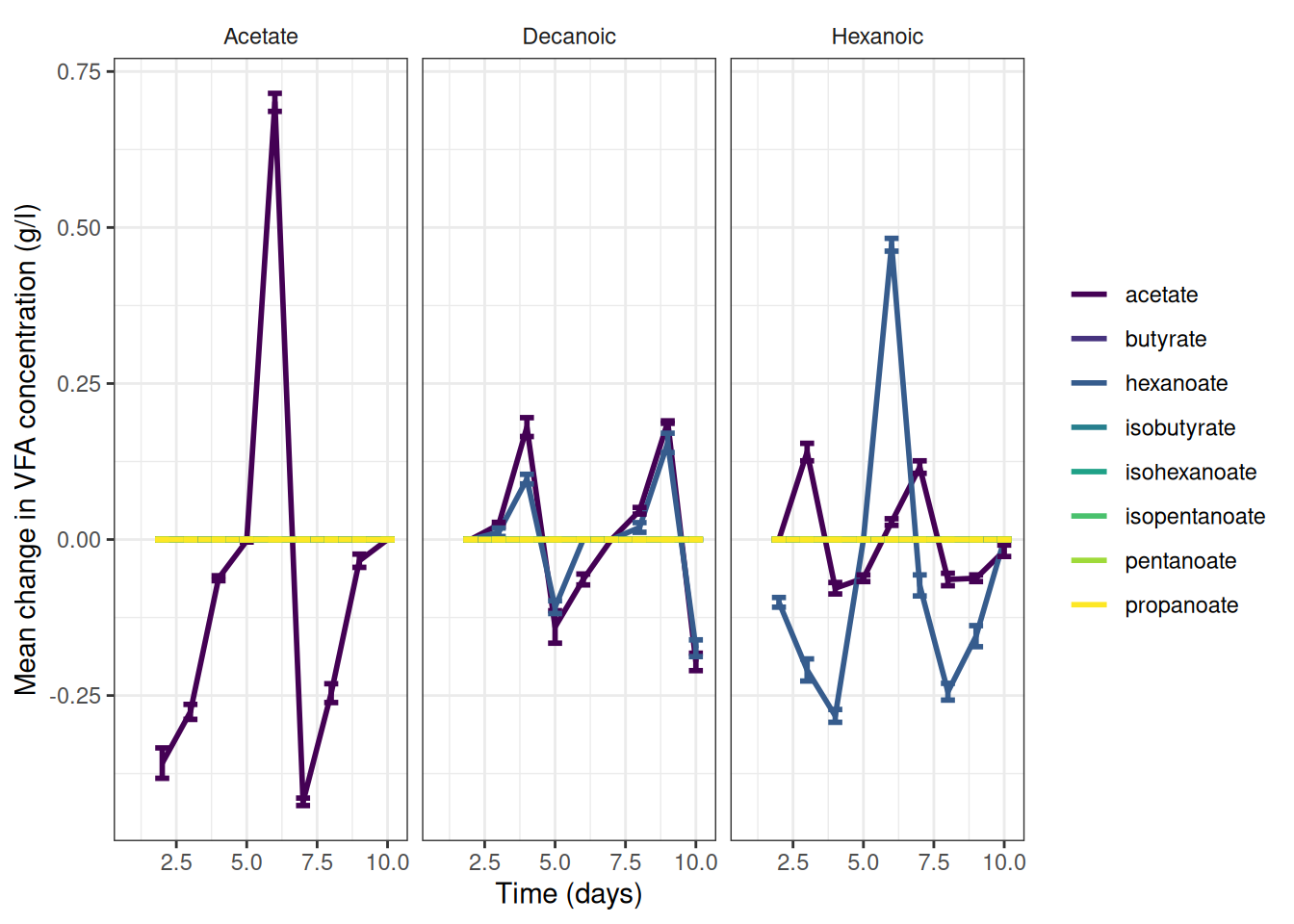
🎬 Graph the change data, grams per litre:
vfa_delta_summary |>
  ggplot(aes(x = time_day, colour = vfa)) +
  geom_line(aes(y = mean_g_l),
            linewidth = 1) +
  geom_errorbar(aes(ymin = mean_g_l - se_g_l,
                    ymax = mean_g_l + se_g_l),
                width = 0.5,
                show.legend = F,
                linewidth = 1) +
  scale_color_viridis_d(name = NULL) +
  scale_x_continuous(name = "Time (days)") +
  scale_y_continuous(name = "Mean change in VFA concentration (g/l)") +
  theme_bw() +
  facet_wrap(~treatment) +
  theme(strip.background = element_blank())
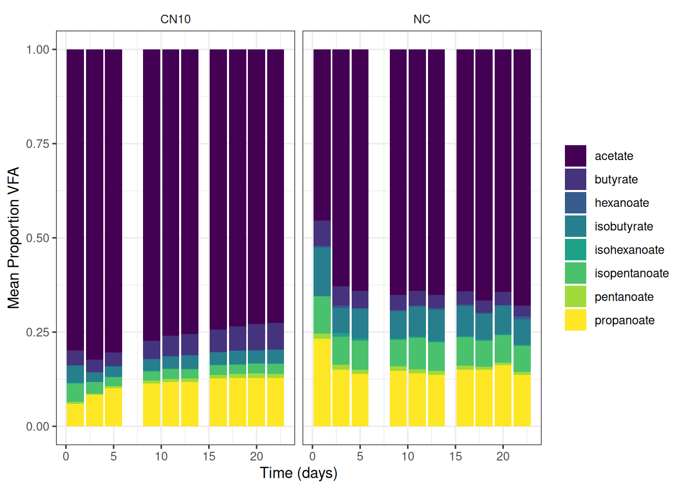
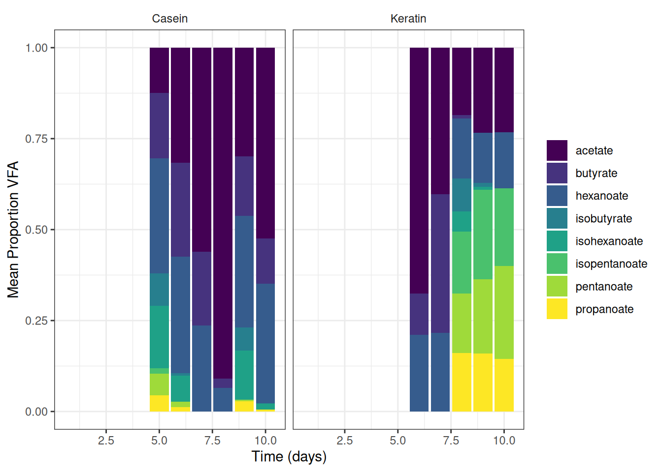
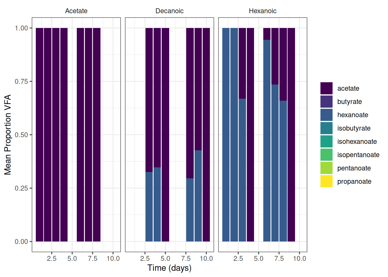
🎬 Graph the mean percent representation of each VFA g/l. Note geom_col() will plot proportion if we setposition = "fill"
vfa_cummul_summary |>
  ggplot(aes(x = time_day, y = mean_g_l, fill = vfa)) +
  geom_col(position = "fill") +
  scale_fill_viridis_d(name = NULL) +
  scale_x_continuous(name = "Time (days)") +
  scale_y_continuous(name = "Mean Proportion VFA") +
  theme_bw() +
  facet_wrap(~treatment) +
  theme(strip.background = element_blank())
View the relationship between samples using PCA
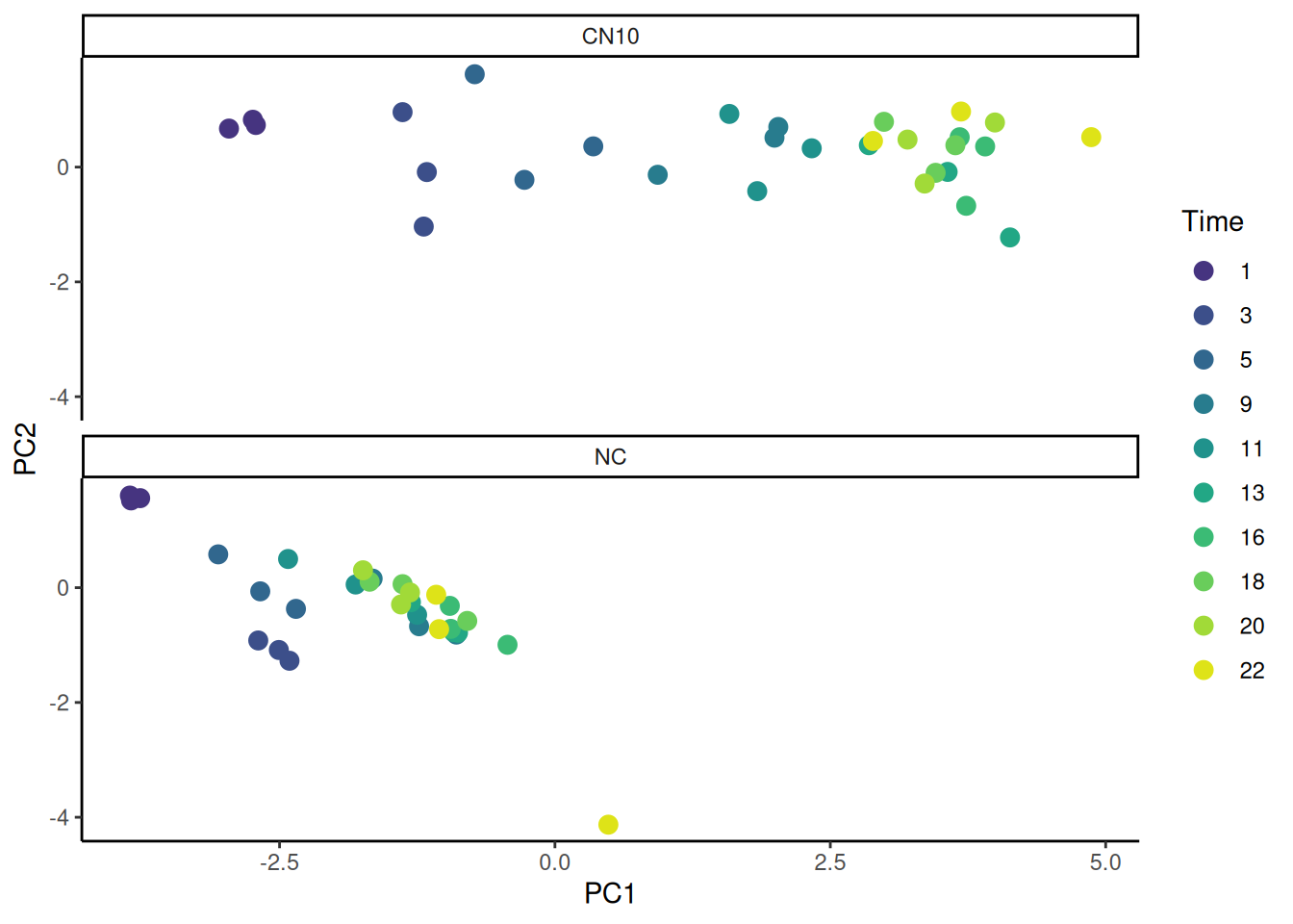
We have 8 VFA in our dataset. PCA will allow us to plot our samples in the “VFA” space so we can see if treatments, time or replicate cluster.
However, PCA expects a matrix with samples in rows and VFA, the variables, in columns. We will need to select the columns we need and pivot wider. Then convert to a matrix.
🎬
vfa_cummul_pca <- vfa_cummul |>
  select(sample_replicate,
         treatment,
         replicate,
         time_day,
         vfa,
         conc_g_l) |>
  pivot_wider(names_from = vfa,
values_from = conc_g_l)🎬 Perform PCA on the matrix:
pca <- mat |>
  prcomp(scale. = TRUE,
         rank. = 4)
The scale. argument tells prcomp() to scale the data to have a mean of 0 and a standard deviation of 1. The rank. argument tells prcomp() to only calculate the first 4 principal components. This is useful for visualisation as we can only plot in 2 or 3 dimensions. We can see the results of the PCA by viewing the summary() of the pca object.
summary(pca)Importance of first k=4 (out of 8) components:
PC1 PC2 PC3 PC4
Standard deviation 2.4977 0.9026 0.77959 0.45567
Proportion of Variance 0.7798 0.1018 0.07597 0.02595
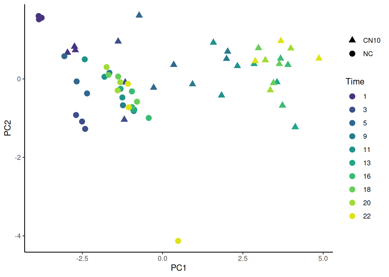
Cumulative Proportion 0.7798 0.8816 0.95760 0.98355The Proportion of Variance tells us how much of the variance is explained by each component. We can see that the first component explains 0.7798 of the variance, the second 0.1018, and the third 0.07597. Together the first three components explain nearly 96% of the total variance in the data. Plotting PC1 against PC2 will capture about 78% of the variance which is likely much better than we would get plotting any two VFA against each other. To plot the PC1 against PC2 we will need to extract the PC1 and PC2 score from the pca object and add labels for the samples.
🎬 Create a dataframe of the PC1 and PC2 scores which are in pca$x and add the sample information from vfa_cummul_pca:
pca_labelled <- data.frame(pca$x,
                           sample_replicate = vfa_cummul_pca$sample_replicate,
                           treatment = vfa_cummul_pca$treatment,
                           replicate = vfa_cummul_pca$replicate,
                           time_day = vfa_cummul_pca$time_day)
The dataframe should look like this:
| PC1 | PC2 | PC3 | PC4 | sample_replicate | treatment | replicate | time_day |
|---|---|---|---|---|---|---|---|
| -2.9592362 | 0.6710553 | 0.0068846 | -0.4453904 | CN10-1 | CN10 | 1 | 1 |
| -2.7153060 | 0.7338367 | -0.2856872 | -0.2030110 | CN10-2 | CN10 | 2 | 1 |
| -2.7423102 | 0.8246832 | -0.4964249 | -0.1434490 | CN10-3 | CN10 | 3 | 1 |
| -1.1909064 | -1.0360724 | 1.1249513 | -0.7360599 | CN10-1 | CN10 | 1 | 3 |
| -1.3831563 | 0.9572091 | -1.5561657 | 0.0582755 | CN10-2 | CN10 | 2 | 3 |
| -1.1628940 | -0.0865412 | -0.6046780 | -0.1976743 | CN10-3 | CN10 | 3 | 3 |
| -0.2769661 | -0.2221055 | 1.1579897 | -0.6079395 | CN10-1 | CN10 | 1 | 5 |
| 0.3480962 | 0.3612522 | 0.5841649 | -0.0612366 | CN10-2 | CN10 | 2 | 5 |
| -0.7281116 | 1.6179706 | -0.6430170 | 0.0660727 | CN10-3 | CN10 | 3 | 5 |
| 0.9333578 | -0.1339061 | 1.0870945 | -0.4374103 | CN10-1 | CN10 | 1 | 9 |
| 2.0277528 | 0.6993342 | 0.3850147 | 0.0723540 | CN10-2 | CN10 | 2 | 9 |
| 1.9931908 | 0.5127260 | 0.6605782 | 0.1841974 | CN10-3 | CN10 | 3 | 9 |
| 1.8365692 | -0.4189762 | 0.7029015 | -0.3873133 | CN10-1 | CN10 | 1 | 11 |
| 2.3313978 | 0.3274834 | -0.0135608 | 0.0264372 | CN10-2 | CN10 | 2 | 11 |
| 1.5833035 | 0.9263509 | -0.1909483 | 0.1358320 | CN10-3 | CN10 | 3 | 11 |
| 2.8498246 | 0.3815854 | -0.4763500 | -0.0280281 | CN10-1 | CN10 | 1 | 13 |
| 3.5652461 | -0.0836709 | -0.5948483 | -0.1612809 | CN10-2 | CN10 | 2 | 13 |
| 4.1314944 | -1.2254642 | 0.2699666 | -0.3152100 | CN10-3 | CN10 | 3 | 13 |
| 3.7338024 | -0.6744610 | 0.4344639 | -0.3736234 | CN10-1 | CN10 | 1 | 16 |
| 3.6748427 | 0.5202498 | -0.4333685 | -0.1607235 | CN10-2 | CN10 | 2 | 16 |
| 3.9057053 | 0.3599520 | -0.3049074 | 0.0540037 | CN10-3 | CN10 | 3 | 16 |
| 3.4561583 | -0.0996639 | 0.4472090 | -0.0185889 | CN10-1 | CN10 | 1 | 18 |
| 3.6354729 | 0.3809673 | -0.0934957 | 0.0018722 | CN10-2 | CN10 | 2 | 18 |
| 2.9872250 | 0.7890400 | -0.2361098 | -0.1628506 | CN10-3 | CN10 | 3 | 18 |
| 3.3562231 | -0.2866224 | 0.1331068 | -0.2056366 | CN10-1 | CN10 | 1 | 20 |
| 3.2009943 | 0.4795967 | -0.2092384 | -0.5962183 | CN10-2 | CN10 | 2 | 20 |
| 3.9948127 | 0.7772640 | -0.3181372 | 0.1218382 | CN10-3 | CN10 | 3 | 20 |
| 2.8874207 | 0.4554681 | 0.3106044 | -0.2220240 | CN10-1 | CN10 | 1 | 22 |
| 3.6868864 | 0.9681097 | -0.2174166 | -0.2246775 | CN10-2 | CN10 | 2 | 22 |
| 4.8689622 | 0.5218563 | -0.2906042 | 0.3532981 | CN10-3 | CN10 | 3 | 22 |
| -3.8483418 | 1.5205541 | -0.8809715 | -0.5306228 | NC-1 | NC | 1 | 1 |
| -3.7653460 | 1.5598499 | -1.0570798 | -0.4075397 | NC-2 | NC | 2 | 1 |
| -3.8586309 | 1.6044929 | -1.0936576 | -0.4292404 | NC-3 | NC | 3 | 1 |
| -2.6934553 | -0.9198406 | 0.7439841 | -0.9881115 | NC-1 | NC | 1 | 3 |
| -2.5064076 | -1.0856761 | 0.6334250 | -0.8999028 | NC-2 | NC | 2 | 3 |
| -2.4097945 | -1.2731546 | 1.1767665 | -0.8715948 | NC-3 | NC | 3 | 3 |
| -3.0567309 | 0.5804906 | -0.1391344 | -0.3701763 | NC-1 | NC | 1 | 5 |
| -2.3511737 | -0.3692016 | 0.7053757 | -0.3284113 | NC-2 | NC | 2 | 5 |
| -2.6752311 | -0.0637855 | 0.4692194 | -0.3841240 | NC-3 | NC | 3 | 5 |
| -1.2335368 | -0.6717374 | 0.2155285 | 0.1060486 | NC-1 | NC | 1 | 9 |
| -1.6550689 | 0.1576557 | 0.0687658 | 0.2750388 | NC-2 | NC | 2 | 9 |
| -0.8948103 | -0.8171884 | 0.8062876 | 0.5032756 | NC-3 | NC | 3 | 9 |
| -1.2512737 | -0.4720993 | 0.4071788 | 0.4693106 | NC-1 | NC | 1 | 11 |
| -1.8091407 | 0.0552546 | 0.0424090 | 0.3918222 | NC-2 | NC | 2 | 11 |
| -2.4225566 | 0.4998948 | -0.1987773 | 0.1959282 | NC-3 | NC | 3 | 11 |
| -0.9193427 | -0.7741826 | 0.0918984 | 0.5089847 | NC-1 | NC | 1 | 13 |
| -0.8800183 | -0.7850404 | 0.0895146 | 0.6050052 | NC-2 | NC | 2 | 13 |
| -1.3075763 | -0.2525829 | -0.2993318 | 0.5874269 | NC-3 | NC | 3 | 13 |
| -0.9543813 | -0.3170305 | 0.0885062 | 0.7153071 | NC-1 | NC | 1 | 16 |
| -0.4303679 | -0.9952374 | 0.2038883 | 0.8214647 | NC-2 | NC | 2 | 16 |
| -0.9457300 | -0.7180646 | 0.3081282 | 0.6563748 | NC-3 | NC | 3 | 16 |
| -1.3830063 | 0.0614677 | -0.2805342 | 0.5462137 | NC-1 | NC | 1 | 18 |
| -0.7960522 | -0.5792768 | -0.0369684 | 0.6621526 | NC-2 | NC | 2 | 18 |
| -1.6822927 | 0.1041656 | 0.0634251 | 0.4337240 | NC-3 | NC | 3 | 18 |
| -1.3157478 | -0.0835664 | -0.1246253 | 0.5599467 | NC-1 | NC | 1 | 20 |
| -1.7425068 | 0.3029227 | -0.0161466 | 0.5134360 | NC-2 | NC | 2 | 20 |
| -1.3970678 | -0.2923056 | 0.4324586 | 0.4765460 | NC-3 | NC | 3 | 20 |
| -1.0777451 | -0.1232925 | 0.2388682 | 0.7585307 | NC-1 | NC | 1 | 22 |
| 0.4851039 | -4.1291445 | -4.0625050 | -0.4582436 | NC-2 | NC | 2 | 22 |
| -1.0516226 | -0.7228479 | 1.0641320 | 0.4955951 | NC-3 | NC | 3 | 22 |
🎬 Plot PC1 against PC2 and colour by time and shape by treatment:
pca_labelled |>
  ggplot(aes(x = PC1, y = PC2,
             colour = factor(time_day),
             shape = treatment)) +
  geom_point(size = 3) +
  scale_colour_viridis_d(end = 0.95, begin = 0.15,
                         name = "Time") +
  scale_shape_manual(values = c(17, 19),
                     name = NULL) +
  theme_classic()
🎬 Plot PC1 against PC2 and colour by time and facet treatment:
pca_labelled |>
  ggplot(aes(x = PC1, y = PC2, colour = factor(time_day))) +
  geom_point(size = 3) +
  scale_colour_viridis_d(end = 0.95, begin = 0.15,
                         name = "Time") +
  facet_wrap(~treatment, ncol = 1) +
  theme_classic()
replicates are similar at the same time and treatment especially early as we might expect. PC is essentially an axis of time.
Visualise the VFA concentration using a heatmap
We are going to create an interactive heatmap with the heatmaply (Galili et al. 2017) package. heatmaply takes a matrix as input so we can use mat
🎬 Set the rownames to the sample id whihcih is combination of sample_replicate and time_day:
rownames(mat) <- interaction(vfa_cummul_pca$sample_replicate,
                             vfa_cummul_pca$time_day)
You might want to view the matrix by clicking on it in the environment pane.
🎬 Load the heatmaply package:
We need to tell the clustering algorithm how many clusters to create. We will set the number of clusters for the treatments to be 2 and the number of clusters for the vfa to be the same since it makes sense to see what clusters of genes correlate with the treatments.
🎬 Set the number of clusters for the treatments and vfa:
n_treatment_clusters <- 2
n_vfa_clusters <- 2
🎬 Create the heatmap:
heatmaply(mat,
          scale = "column",
          k_col = n_vfa_clusters,
          k_row = n_treatment_clusters,
          fontsize_row = 7, fontsize_col = 10,
          labCol = colnames(mat),
          labRow = rownames(mat),
          heatmap_layers = theme(axis.line = element_blank()))
The heatmap will open in the viewer pane (rather than the plot pane) because it is html. You can “Show in a new window” to see it in a larger format. You can also zoom in and out and pan around the heatmap and download it as a png. You might feel the colour bars is not adding much to the plot. You can remove it by setting hide_colorbar = TRUE, in the heatmaply() function.
One of the NC replicates at time = 22 is very different from the other replicates. The CN10 treatments cluster together at high time points. CN10 samples are more similar to NC samples early on. Most of the VFAs behave similarly with highest values later in the experiment for CN10 but isohexanoate and hexanoate differ. The difference might be because isohexanoate is especially low in the NC replicates at time = 1 and hexanoate is especially high in the NC replicate 2 at time = 22
4. Calculate the flux
Calculate the flux(change in VFA concentration over a period of time, divided by weight or volume of material) of each VFA, by mM and by weight. Emma’s note: I think the terms flux and reaction rate are used interchangeably
I’ve requested clarification: for the flux measurements, do they need graphs of the rate of change wrt time? And is the sludge volume going to be a constant for all samples or something they measure and varies by vial?
Answer: The sludge volume is constant, at 30 mls within a 120ml vial. Some students will want to graph reaction rate with time, others will want to compare the measured GC-FID concentrations against the model output.
📢 Kelly asked for “.. a simple flux measurement, which is the change in VFA concentration over a period of time, divided by weight or volume of material. In this case it might be equal to == Delta(Acetate at 3 days - Acetate at 1 day)/Delta (3days - 1day)/50 mls sludge. This would provide a final flux with the units of mg acetate per ml sludge per day.”
Note: Kelly says mg/ml where earlier he used g/L. These are the same (but I called my column conc_g_l)
We need to use the vfa_delta data frame. It contains the change in VFA concentration and the change in time. We will add a column for the flux of each VFA in g/L/day. (mg/ml/day)
sludge_volume <- 30 # ml
vfa_delta <- vfa_delta |>
  mutate(flux = conc_g_l / delta_time / sludge_volume)
NAs at time 1 are expected because there’s no time before that to calculate a changes
5. Graph and extract the reaction rate - pending
Graph and extract the reaction rate assuming a first order chemical/biological reaction and an exponential falloff rate
I’ve requested clarification: for the nonlinear least squares curve fitting, I assume x is time but I’m not clear what the Y variable is - concentration? or change in concentration? or rate of change of concentration?
Answer: The non-linear equation describes concentration change with time. Effectively the change in concentration is dependent upon the available concentration, in this example [Hex] represents the concentration of Hexanoic acid, while the T0 and T1 represent time steps.
[Hex]T1 = [Hex]T0 - [Hex]T0 * k
Or. the amount of Hexanoic acid remaining at T1 (let’s say one hour from the last data point) is equal to the starting concentration ([Hex]T0) minus the concentration dependent metabolism ([Hex]To * k).
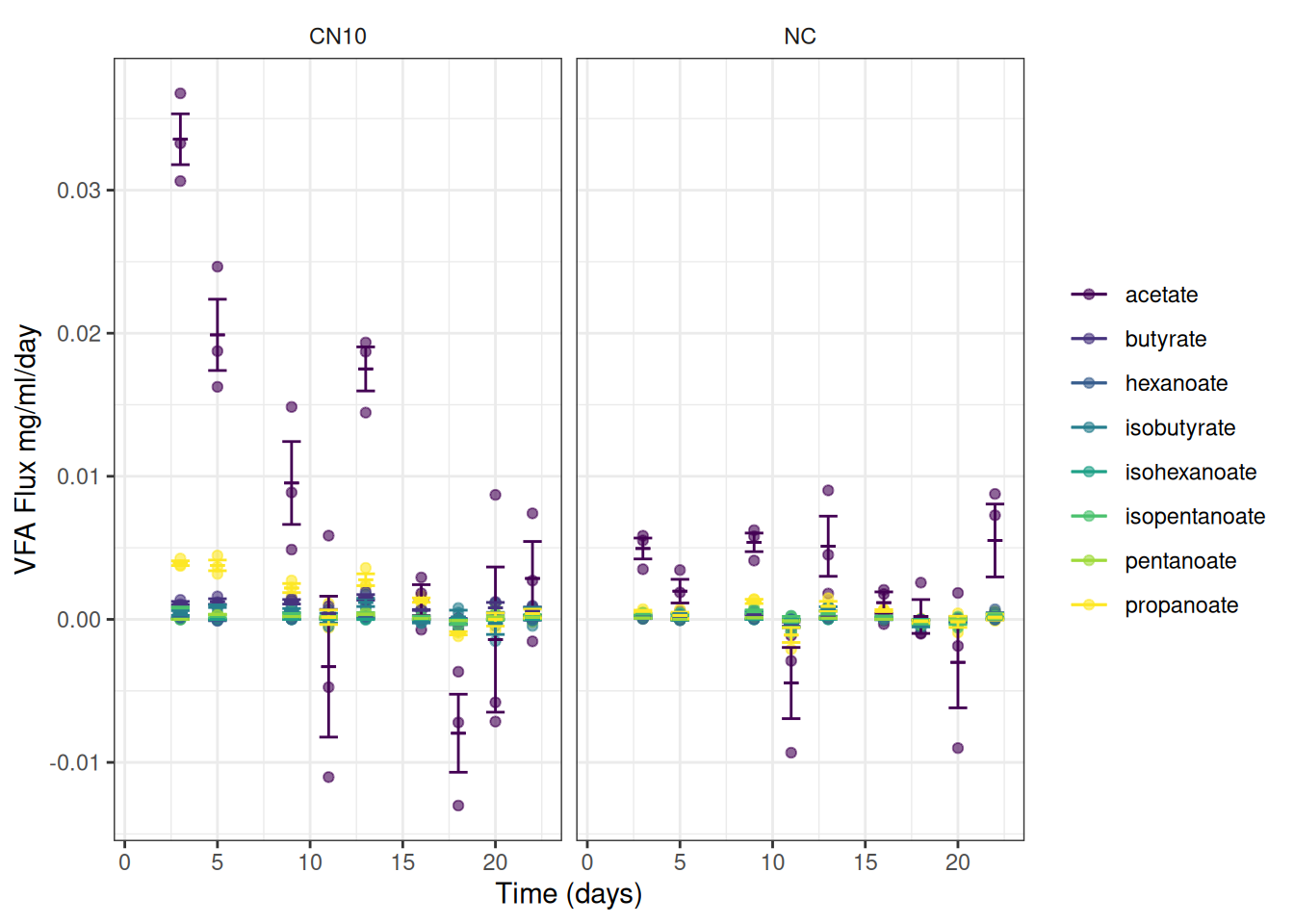
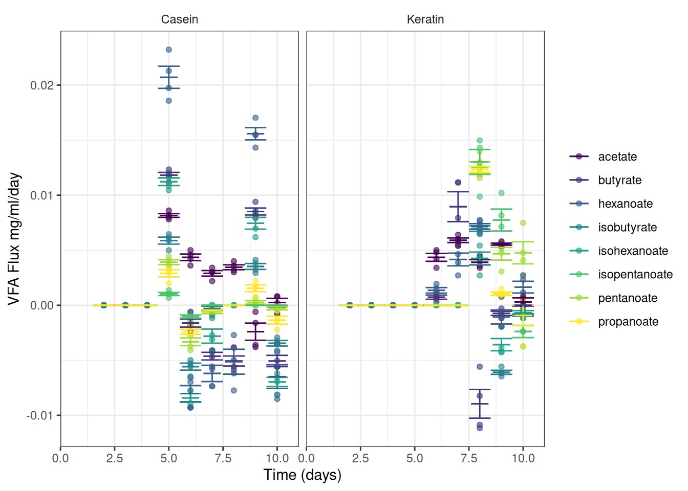
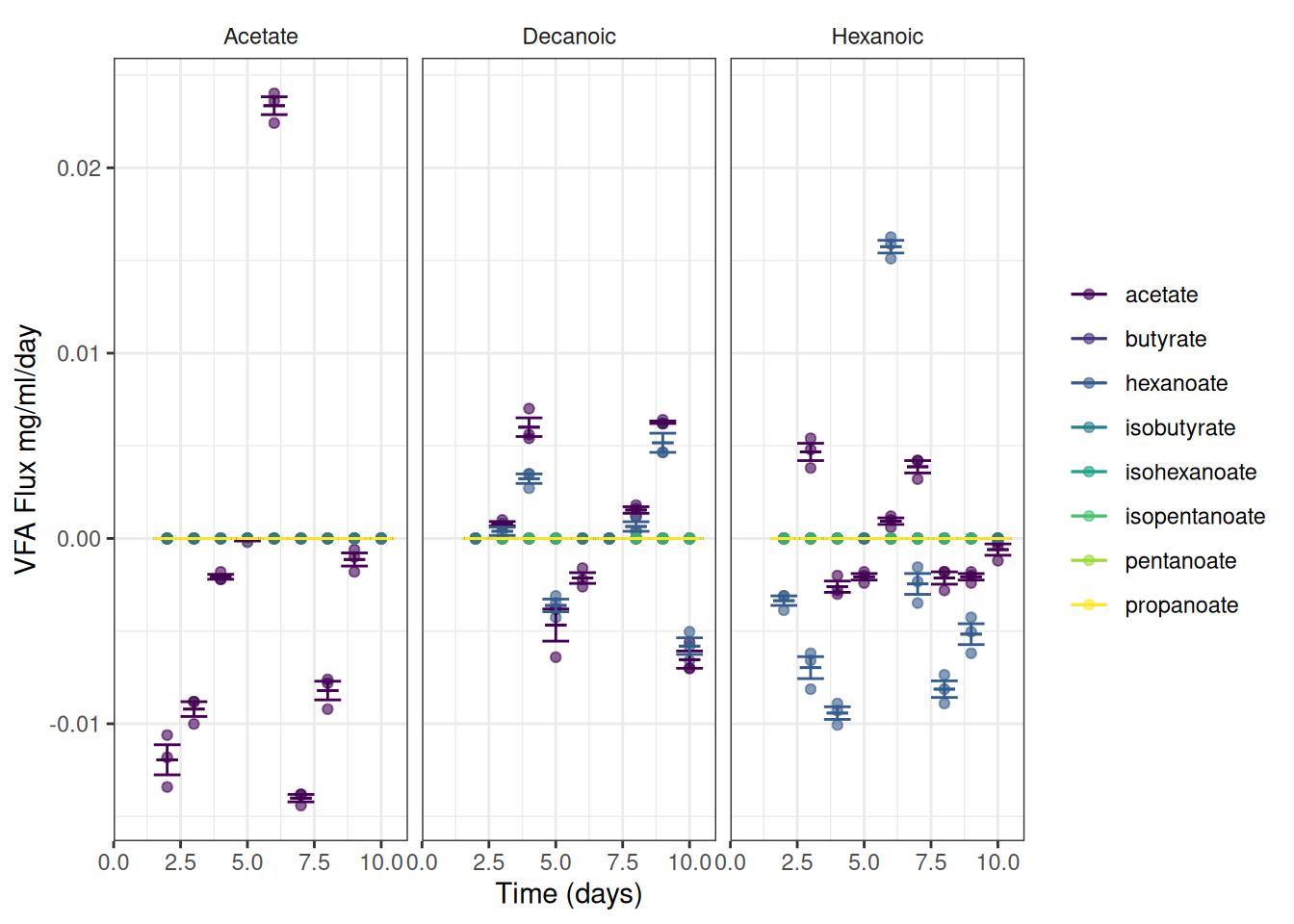
📢 We can now plot the observed fluxes (reaction rates) over time
I’ve summarised the data to add error bars and means
ggplot(data = vfa_delta, aes(x = time_day, colour = vfa)) +
  geom_point(aes(y = flux), alpha = 0.6) +
  geom_errorbar(data = vfa_delta_summary,
                aes(ymin = mean_flux - se_flux,
                    ymax = mean_flux + se_flux),
                width = 1) +
  geom_errorbar(data = vfa_delta_summary,
                aes(ymin = mean_flux,
                    ymax = mean_flux),
                width = 0.8) +
  scale_color_viridis_d(name = NULL) +
  scale_x_continuous(name = "Time (days)") +
  scale_y_continuous(name = "VFA Flux mg/ml/day") +
  theme_bw() +
  facet_wrap(~treatment) +
  theme(strip.background = element_blank())
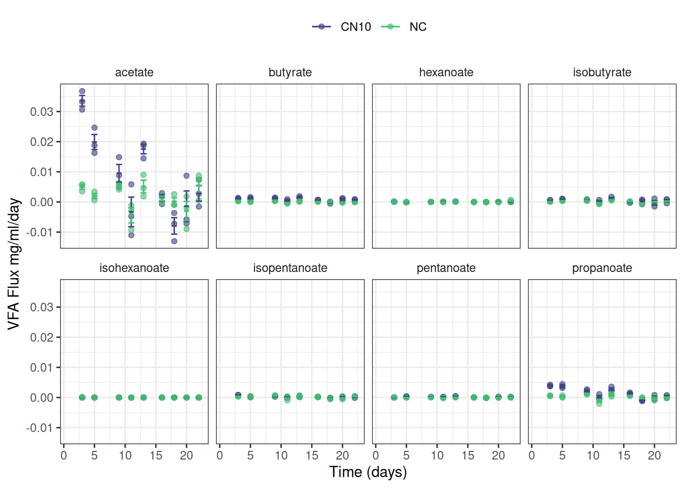
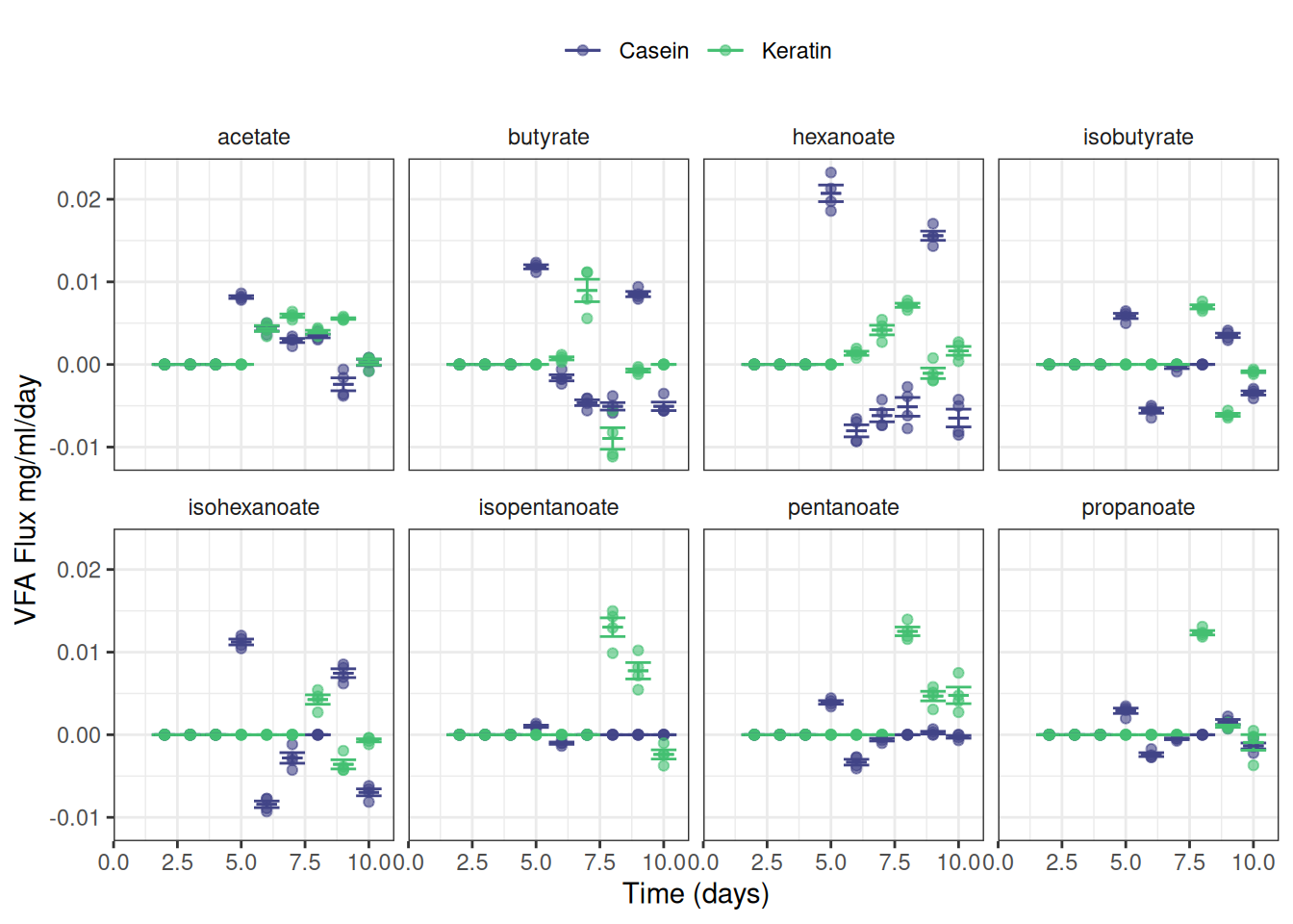
Or maybe this is easier to read:
ggplot(data = vfa_delta, aes(x = time_day, colour = treatment)) +
  geom_point(aes(y = flux), alpha = 0.6) +
  geom_errorbar(data = vfa_delta_summary,
                aes(ymin = mean_flux - se_flux,
                    ymax = mean_flux + se_flux),
                width = 1) +
  geom_errorbar(data = vfa_delta_summary,
                aes(ymin = mean_flux,
                    ymax = mean_flux),
                width = 0.8) +
  scale_color_viridis_d(name = NULL, begin = 0.2, end = 0.7) +
  scale_x_continuous(name = "Time (days)") +
  scale_y_continuous(name = "VFA Flux mg/ml/day") +
  theme_bw() +
  facet_wrap(~ vfa, nrow = 2) +
  theme(strip.background = element_blank(),
        legend.position = "top")
I have not yet worked out the best way to plot the modelled reaction rate
Workflow 2024-04-04
This workflow has been written for the data files I now have! Bear in mind that what you might need from here is going to depend on the narrative of your report. You only need include in the compendium things that support your report.
These are the two files I have
I fixed some inconsistent formatting and unhelpful naming (sigh!) and down loaded these as csv files and saved them in the data-raw folder as:
We also have the Molecular weights for each VFA in grams per mole mol_wt.txt
I recommend restarting R before you start this workflow: Control-Shift-F10 (or use the Session menu)
VFA data
🎬 Load packages
vfa_cummul <- read_csv("data-raw/vfa2.csv") |> janitor::clean_names()This what I think we have:
set_number Two data sets, one about VFA treatment (2) and one about Protein treatments (1)
-
replicate
- for set 1: 1-4
- for set 2: 1-3
-
treatment
- for set 1: Casein, Keratin
- for set 2: Acetate, Hexanoic, Decanoic
time_day time in days (note time in the ph data in in hours)
then columns for each of the 8 measured VFA: acetate, propanoate, isobutyrate, butyrate, isopentanoate, pentanoate, isohexanoate, hexanoate
I think some of the data have been mislabelled as set 2 when it is set 1. I changed these in the csv file but not on the google sheet until someone can confirm there really are mislabelled).
I’m going to split these into the two data sets and work on them separately
🎬 Split the data into the two sets. Note we also remove the set number column as it isn’t need if the data is split into the two sets.
vfa_cummul_protein has 2 treatments, four replicates and 10 days = 2 x 4 x 10 = 80 rows
vfa_cummul_vfa has 3 treatments, 3 replicates and 10 days = 3 x 3 x 10 = 90 rows
🎬 import molecular weight data
mol_wt <- read_table("data-raw/mol_wt.txt") |>
  mutate(vfa = tolower(vfa))
Set 1: Protein treatments
1. Calculate Change in VFA g/l with time
🎬 Create dataframe for the change in VFA the change in time
vfa_delta_protein <- vfa_cummul_protein |>
    group_by(treatment, replicate)  |>
    arrange(treatment, replicate, time_day) |>
    mutate(acetate = acetate - lag(acetate),
           propanoate = propanoate - lag(propanoate),
           isobutyrate = isobutyrate - lag(isobutyrate),
           butyrate = butyrate - lag(butyrate),
           isopentanoate = isopentanoate - lag(isopentanoate),
           pentanoate = pentanoate - lag(pentanoate),
           isohexanoate = isohexanoate - lag(isohexanoate),
           hexanoate = hexanoate - lag(hexanoate),
           delta_time = time_day - lag(time_day))
Now we have two dataframes, one for the cumulative data and one for the change in VFA and time. Note that the VFA values have been replaced by the change in VFA but the change in time is in a separate column. I have done this because we later want to plot flux. Note that unlike the sample data, the time steps are all 1 day so the change in time is always 1 and not really needed. I have included it here to make more clear that the units of flux are which is the change in VFA concentration per unit of time per unit of weight or volume of material
2. Recalculate the data into grams per litre
To make conversions from mM to g/l we need to do mM * 0.001 * MW. We will pivot the VFA data to long format and join the molecular weight data to the VFA data. Then we can calculate the g/l. We will do this for both the cumulative and delta dataframes.
🎬 Pivot the cumulative data to long format:
vfa_cummul_protein <- vfa_cummul_protein |>
  pivot_longer(cols = -c(treatment,
                         replicate,
                         time_day),
               values_to = "conc_mM",
               names_to = "vfa")
View vfa_cummul_protein to check you understand what you have done.
🎬 Join molecular weight to data and calculate g/l (mutate to convert to g/l * 0.001 * MW):
View vfa_cummul_protein to check you understand what you have done.
Repeat for the delta data.
🎬 Pivot the change data, vfa_delta_protein to long format (📢 delta_time is added to the list of columns that do not need to be pivoted but repeated):
vfa_delta_protein <- vfa_delta_protein |>
  pivot_longer(cols = -c(treatment,
                         replicate,
                         time_day,
                         delta_time),
               values_to = "conc_mM",
               names_to = "vfa")
View vfa_delta_protein to check it looks like vfa_cummul_protein.
🎬 Join molecular weight to data and calculate g/l (mutate to convert to g/l * 0.001 * MW):
3. Calculate the percent representation of each VFA
by mM and by weight
🎬 Add a column which is the percent representation of each VFA for mM and g/l:
Graphs for info so far
🎬 Make summary data for graphing
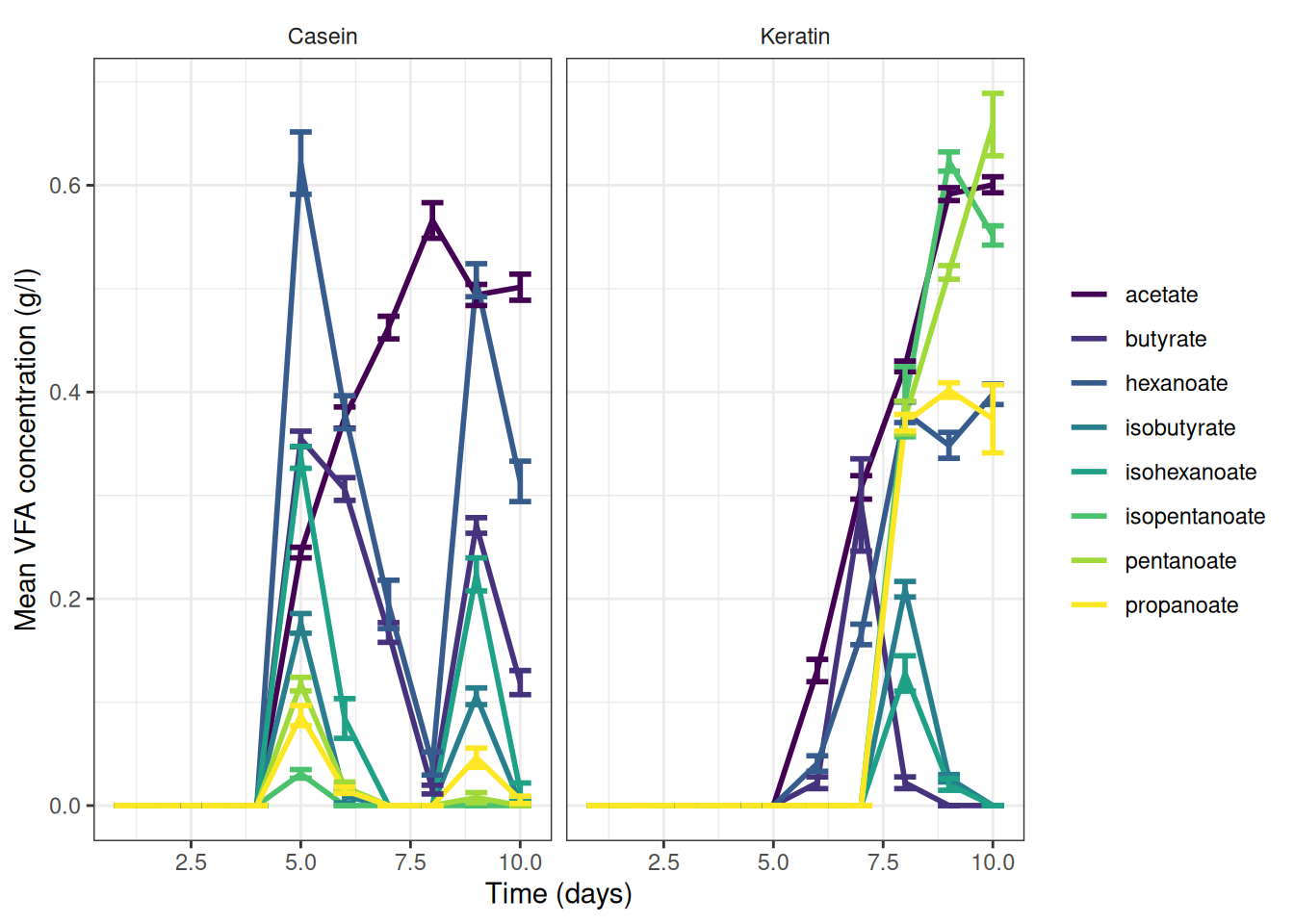
🎬 Graph the cumulative data, grams per litre:
vfa_cummul_protein_summary |>
  ggplot(aes(x = time_day, colour = vfa)) +
  geom_line(aes(y = mean_g_l),
            linewidth = 1) +
  geom_errorbar(aes(ymin = mean_g_l - se_g_l,
                    ymax = mean_g_l + se_g_l),
                width = 0.5,
                show.legend = F,
                linewidth = 1) +
  scale_color_viridis_d(name = NULL) +
  scale_x_continuous(name = "Time (days)") +
  scale_y_continuous(name = "Mean VFA concentration (g/l)") +
  theme_bw() +
  facet_wrap(~treatment) +
  theme(strip.background = element_blank())
🎬 Graph the change data, grams per litre:
vfa_delta_protein_summary |>
  ggplot(aes(x = time_day, colour = vfa)) +
  geom_line(aes(y = mean_g_l),
            linewidth = 1) +
  geom_errorbar(aes(ymin = mean_g_l - se_g_l,
                    ymax = mean_g_l + se_g_l),
                width = 0.5,
                show.legend = F,
                linewidth = 1) +
  scale_color_viridis_d(name = NULL) +
  scale_x_continuous(name = "Time (days)") +
  scale_y_continuous(name = "Mean change in VFA concentration (g/l)") +
  theme_bw() +
  facet_wrap(~treatment) +
  theme(strip.background = element_blank())
🎬 Graph the mean percent representation of each VFA g/l. Note geom_col() will plot proportion if we setposition = "fill"
vfa_cummul_protein_summary |>
  ggplot(aes(x = time_day, y = mean_g_l, fill = vfa)) +
  geom_col(position = "fill") +
  scale_fill_viridis_d(name = NULL) +
  scale_x_continuous(name = "Time (days)") +
  scale_y_continuous(name = "Mean Proportion VFA") +
  theme_bw() +
  facet_wrap(~treatment) +
  theme(strip.background = element_blank())
4. Calculate the flux
Calculate the flux(change in VFA concentration over a period of time, divided by weight or volume of material) of each VFA, by mM and by weight. Emma’s note: I think the terms flux and reaction rate are used interchangeably
The sludge volume is constant, at 30 mls. Flux units are mg vfa per ml sludge per day
Note: Kelly says mg/ml where earlier he used g/L. These are the same (but I called my column conc_g_l)
We need to use the vfa_delta_protein data frame. It contains the change in VFA concentration and the change in time. We will add a column for the flux of each VFA in g/L/day. (mg/ml/day)
sludge_volume <- 30 # ml
vfa_delta_protein <- vfa_delta_protein |>
  mutate(flux = conc_g_l / delta_time / sludge_volume)
NAs at time 1 are expected because there’s no time before that to calculate a changes
5. Graph and extract the reaction rate
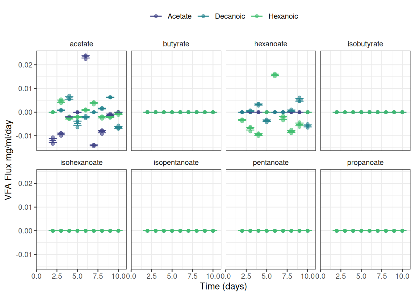
We can now plot the observed fluxes (reaction rates) over time
I’ve summarised the data to add error bars and means
ggplot(data = vfa_delta_protein, aes(x = time_day, colour = vfa)) +
  geom_point(aes(y = flux), alpha = 0.6) +
  geom_errorbar(data = vfa_delta_protein_summary,
                aes(ymin = mean_flux - se_flux,
                    ymax = mean_flux + se_flux),
                width = 1) +
  geom_errorbar(data = vfa_delta_protein_summary,
                aes(ymin = mean_flux,
                    ymax = mean_flux),
                width = 0.8) +
  scale_color_viridis_d(name = NULL) +
  scale_x_continuous(name = "Time (days)") +
  scale_y_continuous(name = "VFA Flux mg/ml/day") +
  theme_bw() +
  facet_wrap(~treatment) +
  theme(strip.background = element_blank())
Or maybe this is easier to read:
ggplot(data = vfa_delta_protein, aes(x = time_day, colour = treatment)) +
  geom_point(aes(y = flux), alpha = 0.6) +
  geom_errorbar(data = vfa_delta_protein_summary,
                aes(ymin = mean_flux - se_flux,
                    ymax = mean_flux + se_flux),
                width = 1) +
  geom_errorbar(data = vfa_delta_protein_summary,
                aes(ymin = mean_flux,
                    ymax = mean_flux),
                width = 0.8) +
  scale_color_viridis_d(name = NULL, begin = 0.2, end = 0.7) +
  scale_x_continuous(name = "Time (days)") +
  scale_y_continuous(name = "VFA Flux mg/ml/day") +
  theme_bw() +
  facet_wrap(~ vfa, nrow = 2) +
  theme(strip.background = element_blank(),
        legend.position = "top")
Set 2: VFA treatments
1. Calculate Change in VFA g/l with time
🎬 Create dataframe for the change in VFA the change in time
vfa_delta_vfa <- vfa_cummul_vfa |>
    group_by(treatment, replicate)  |>
    arrange(treatment, replicate, time_day) |>
    mutate(acetate = acetate - lag(acetate),
           propanoate = propanoate - lag(propanoate),
           isobutyrate = isobutyrate - lag(isobutyrate),
           butyrate = butyrate - lag(butyrate),
           isopentanoate = isopentanoate - lag(isopentanoate),
           pentanoate = pentanoate - lag(pentanoate),
           isohexanoate = isohexanoate - lag(isohexanoate),
           hexanoate = hexanoate - lag(hexanoate),
           delta_time = time_day - lag(time_day))
Now we have two dataframes, one for the cumulative data and one for the change in VFA and time. Note that the VFA values have been replaced by the change in VFA but the change in time is in a separate column. I have done this because we later want to plot flux. Note that unlike the sample data, the time steps are all 1 day so the change in time is always 1 and not really needed. I have included it here to make more clear that the units of flux are which is the change in VFA concentration per unit of time per unit of weight or volume of material
2. Recalculate the data into grams per litre
To make conversions from mM to g/l we need to do mM * 0.001 * MW. We will pivot the VFA data to long format and join the molecular weight data to the VFA data. Then we can calculate the g/l. We will do this for both the cumulative and delta dataframes.
🎬 Pivot the cumulative data to long format:
vfa_cummul_vfa <- vfa_cummul_vfa |>
  pivot_longer(cols = -c(treatment,
                         replicate,
                         time_day),
               values_to = "conc_mM",
               names_to = "vfa")
View vfa_cummul_vfa to check you understand what you have done.
🎬 Join molecular weight to data and calculate g/l (mutate to convert to g/l * 0.001 * MW):
View vfa_cummul_vfa to check you understand what you have done.
Repeat for the delta data.
🎬 Pivot the change data, vfa_delta_vfa to long format (📢 delta_time is added to the list of columns that do not need to be pivoted but repeated):
vfa_delta_vfa <- vfa_delta_vfa |>
  pivot_longer(cols = -c(treatment,
                         replicate,
                         time_day,
                         delta_time),
               values_to = "conc_mM",
               names_to = "vfa")
View vfa_delta_vfa to check it looks like vfa_cummul_vfa.
🎬 Join molecular weight to data and calculate g/l (mutate to convert to g/l * 0.001 * MW):
3. Calculate the percent representation of each VFA
by mM and by weight
🎬 Add a column which is the percent representation of each VFA for mM and g/l:
Graphs for info so far
🎬 Make summary data for graphing
🎬 Graph the cumulative data, grams per litre:
vfa_cummul_vfa_summary |>
  ggplot(aes(x = time_day, colour = vfa)) +
  geom_line(aes(y = mean_g_l),
            linewidth = 1) +
  geom_errorbar(aes(ymin = mean_g_l - se_g_l,
                    ymax = mean_g_l + se_g_l),
                width = 0.5,
                show.legend = F,
                linewidth = 1) +
  scale_color_viridis_d(name = NULL) +
  scale_x_continuous(name = "Time (days)") +
  scale_y_continuous(name = "Mean VFA concentration (g/l)") +
  theme_bw() +
  facet_wrap(~treatment) +
  theme(strip.background = element_blank())
🎬 Graph the change data, grams per litre:
vfa_delta_vfa_summary |>
  ggplot(aes(x = time_day, colour = vfa)) +
  geom_line(aes(y = mean_g_l),
            linewidth = 1) +
  geom_errorbar(aes(ymin = mean_g_l - se_g_l,
                    ymax = mean_g_l + se_g_l),
                width = 0.5,
                show.legend = F,
                linewidth = 1) +
  scale_color_viridis_d(name = NULL) +
  scale_x_continuous(name = "Time (days)") +
  scale_y_continuous(name = "Mean change in VFA concentration (g/l)") +
  theme_bw() +
  facet_wrap(~treatment) +
  theme(strip.background = element_blank())
🎬 Graph the mean percent representation of each VFA g/l. Note geom_col() will plot proportion if we setposition = "fill"
vfa_cummul_vfa_summary |>
  ggplot(aes(x = time_day, y = mean_g_l, fill = vfa)) +
  geom_col(position = "fill") +
  scale_fill_viridis_d(name = NULL) +
  scale_x_continuous(name = "Time (days)") +
  scale_y_continuous(name = "Mean Proportion VFA") +
  theme_bw() +
  facet_wrap(~treatment) +
  theme(strip.background = element_blank())
4. Calculate the flux
Calculate the flux(change in VFA concentration over a period of time, divided by weight or volume of material) of each VFA, by mM and by weight. Emma’s note: I think the terms flux and reaction rate are used interchangeably
The sludge volume is constant, at 30 mls. Flux units are mg vfa per ml sludge per day
Note: Kelly says mg/ml where earlier he used g/L. These are the same (but I called my column conc_g_l)
We need to use the vfa_delta_vfa data frame. It contains the change in VFA concentration and the change in time. We will add a column for the flux of each VFA in g/L/day. (mg/ml/day)
sludge_volume <- 30 # ml
vfa_delta_vfa <- vfa_delta_vfa |>
  mutate(flux = conc_g_l / delta_time / sludge_volume)
NAs at time 1 are expected because there’s no time before that to calculate a changes
5. Graph and extract the reaction rate
We can now plot the observed fluxes (reaction rates) over time
I’ve summarised the data to add error bars and means
ggplot(data = vfa_delta_vfa, aes(x = time_day, colour = vfa)) +
  geom_point(aes(y = flux), alpha = 0.6) +
  geom_errorbar(data = vfa_delta_vfa_summary,
                aes(ymin = mean_flux - se_flux,
                    ymax = mean_flux + se_flux),
                width = 1) +
  geom_errorbar(data = vfa_delta_vfa_summary,
                aes(ymin = mean_flux,
                    ymax = mean_flux),
                width = 0.8) +
  scale_color_viridis_d(name = NULL) +
  scale_x_continuous(name = "Time (days)") +
  scale_y_continuous(name = "VFA Flux mg/ml/day") +
  theme_bw() +
  facet_wrap(~treatment) +
  theme(strip.background = element_blank())
Or maybe this is easier to read:
ggplot(data = vfa_delta_vfa, aes(x = time_day, colour = treatment)) +
  geom_point(aes(y = flux), alpha = 0.6) +
  geom_errorbar(data = vfa_delta_vfa_summary,
                aes(ymin = mean_flux - se_flux,
                    ymax = mean_flux + se_flux),
                width = 1) +
  geom_errorbar(data = vfa_delta_vfa_summary,
                aes(ymin = mean_flux,
                    ymax = mean_flux),
                width = 0.8) +
  scale_color_viridis_d(name = NULL, begin = 0.2, end = 0.7) +
  scale_x_continuous(name = "Time (days)") +
  scale_y_continuous(name = "VFA Flux mg/ml/day") +
  theme_bw() +
  facet_wrap(~ vfa, nrow = 2) +
  theme(strip.background = element_blank(),
        legend.position = "top")
ph data
Pages made with R (R Core Team 2024), Quarto (Allaire et al. 2024), knitr (Xie 2024, 2015, 2014), kableExtra (Zhu 2021)
