5 Binomial GLM overview

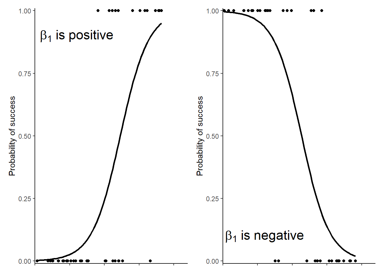
When a response variable can take only one of two values such as 0 and 1, dead and alive, no and yes or failure and success it follows a binomial distribution and can be modelled with a binomial GLM. A binomial GLM is also known as logistic regression. Although the observations themselves can have only one of two values, the scale of the response is a probability representing the probability of 1, alive, yes or success. The link function used in a binomial GLM is the “logit” function also known as “log-odds.” This means the model estimates are also log-odds. This can make it tricky to interpret the estimates but two things can help us. First, the principle about the sign of \(\beta_{1}\) still applies: positive \(\beta_{1}\) indicates an increase in the odds with an increase in \(X1\) and negative \(\beta_{1}\) indicates a decrease in the odds with an increase in \(X1\). See Figure 5.1 for an illustration of the curve for positive and negative \(\beta_{1}\).

Figure 5.1: Data fitted with a binomial GLM.

Second, we can use the predict() function to get values on the scale of the response, a probability, rather than the log-odds. This is easier for most people to understand.

Positive \(\beta_{1}\) indicates an increase in the odds with an increase in \(X1\) and negative \(\beta_{1}\) indicates a decrease in the odds with an increase in \(X1\).

When you have a single explanatory variable, the binomial GLM is:

\[\begin{equation} ln\left(\frac{E(y_{i})}{1-E(y_{i})}\right)=\beta_{0}+\beta_{1}X1_{i} \tag{5.1} \end{equation}\]

This means that the model estimates are odds logged to the base \(e\) and and the inverse function, exp() must be applied to them to interpret as odds.

\[\begin{equation} \frac{E(y_{i})}{1-E(y_{i})}=exp(\beta_{0}+\beta_{1}X1_{i}) \tag{5.2} \end{equation}\]

or

\[\begin{equation} \frac{E(y_{i})}{1-E(y_{i})}=exp(\beta_{0}) \times exp(\beta_{1})^{X1_{i}} \tag{5.3} \end{equation}\]

This looks complicated. Using the predict function because important in reporting the results.

Just like Poisson GLM with a single explanatory variable, there are two parameters in this model, \(\beta_{0}\) and \(\beta_{1}\) and their meaning is similar. Let us assume our response is failure (0) or success (1). Then \(\beta_{0}\) is the log odds of success when the explanatory variable is 0 and \(\beta_{1}\) is the change in the log odds of success for each unit change in the explanatory.

In a binomial GLM the link function is \(logit\) and the estimates are log-odds. Predictions ‘on the scale of the response’ are probabilities of one of the two outcomes.

5.1 What exactly are odds?

An odds is the probability of something happening divided by the probability of it not happening. For example, for a fair coin where heads and tails are equally likely, we can think of the heads as something that happens and tails as it not happening. The odds of a head in a coin toss is:

\(\frac{P(H)}{P( not\:head)} = \frac{0.5}{ 1- 0.5} = 1\)

When the odds are 1, heads and tails are equally likely.

If you had an unfair coin where the probability of a head was \(\frac{3}{4}\) then the odds of a head are:

\(\frac{P(H)}{P( not\:head)} = \frac{0.75}{ 1- 0.75} = 3\)

A head is three times as likely as a tail. When the odds are greater than 1 heads are more probable than tails.

If instead probability of a head was \(\frac{1}{4}\) then the odds of a head are:

\(\frac{P(H)}{P( not\:head)} = \frac{0.25}{ 1- 0.25} = 0.33333\)

A head is a third as likely as a tail. When the odds are less than 1 heads are less probable than tails.

If the odds > 1, success is more likely than failure. If the odds < 1, failure is more likely than success.

5.2 What does this mean for \(\beta_{0}\)?

If our response can be failure (0) or success (1). Then \(\beta_{0}\) is the log odds of success when the explanatory variable is 0. This is:

\[\begin{equation} ln\left(\frac{P(success)}{P(failure)}\right) \tag{5.4} \end{equation}\]

When the probability of success is greater than the probability of failure this will be the log of a number greater than 1 and thus positive. When the probability of success is less than the probability of failure this will be the log of a number less than 1 and thus negative.

Positive \(\beta_{0}\) indicates that the probability of success is greater than the probability of failure at \(x = 0\) and negative \(\beta_{0}\) indicates that the probability of failure is greater than the probability of success at \(x = 0\)

5.3 What does this mean for \(\beta_{1}\)?

\(\beta_{1}\) is the change in the log odds of success for each unit change in the explanatory variable. It is the log of the odds of success at \(x = 1\) divided by the odds of success at \(x = 0\) If the odds of success at \(x = 1\) is greater than the the odds of success at \(x = 0\), this will be log of a number greater than 1 and thus \(\beta_{1}\) is positive. If the odds of success at \(x = 1\) is less than the the odds of success at \(x = 0\), this will be log of a number less than 1 and thus \(\beta_{1}\) is negative.

Positive \(\beta_{1}\) indicates that the probability of success is increasing with \(x\) and negative \(\beta_{1}\) indicates that the probability of success is decreasing with \(x\).