2 Poisson GLM overview
When a response variable is the count of objects, individuals or events it often follows a Poisson distribution. Such variables are always positive - they range from 0 to \(\infty\). A Poisson GLM is also known as Poisson regression. The link function used in a Poisson GLM is the natural logarithm, \(ln\).
When you have a single explanatory variable, that model is:
\[\begin{equation} ln(E(y_{i}))=\beta_{0}+\beta_{1}X1_{i} \tag{2.1} \end{equation}\]
This means that the model estimates are logged to the base \(e\) and and the inverse function, exp() must be applied to them to interpret them in terms of the response. In other words, to make predictions about the expected value of the response we need to exponentiate the coefficients.
\[\begin{equation} E(y_{i})=exp(\beta_{0}+\beta_{1}X1_{i}) \tag{2.2} \end{equation}\]
or
\[\begin{equation} E(y_{i})=exp(\beta_{0}) \times exp(\beta_{1})^{X1_{i}} \tag{2.3} \end{equation}\]
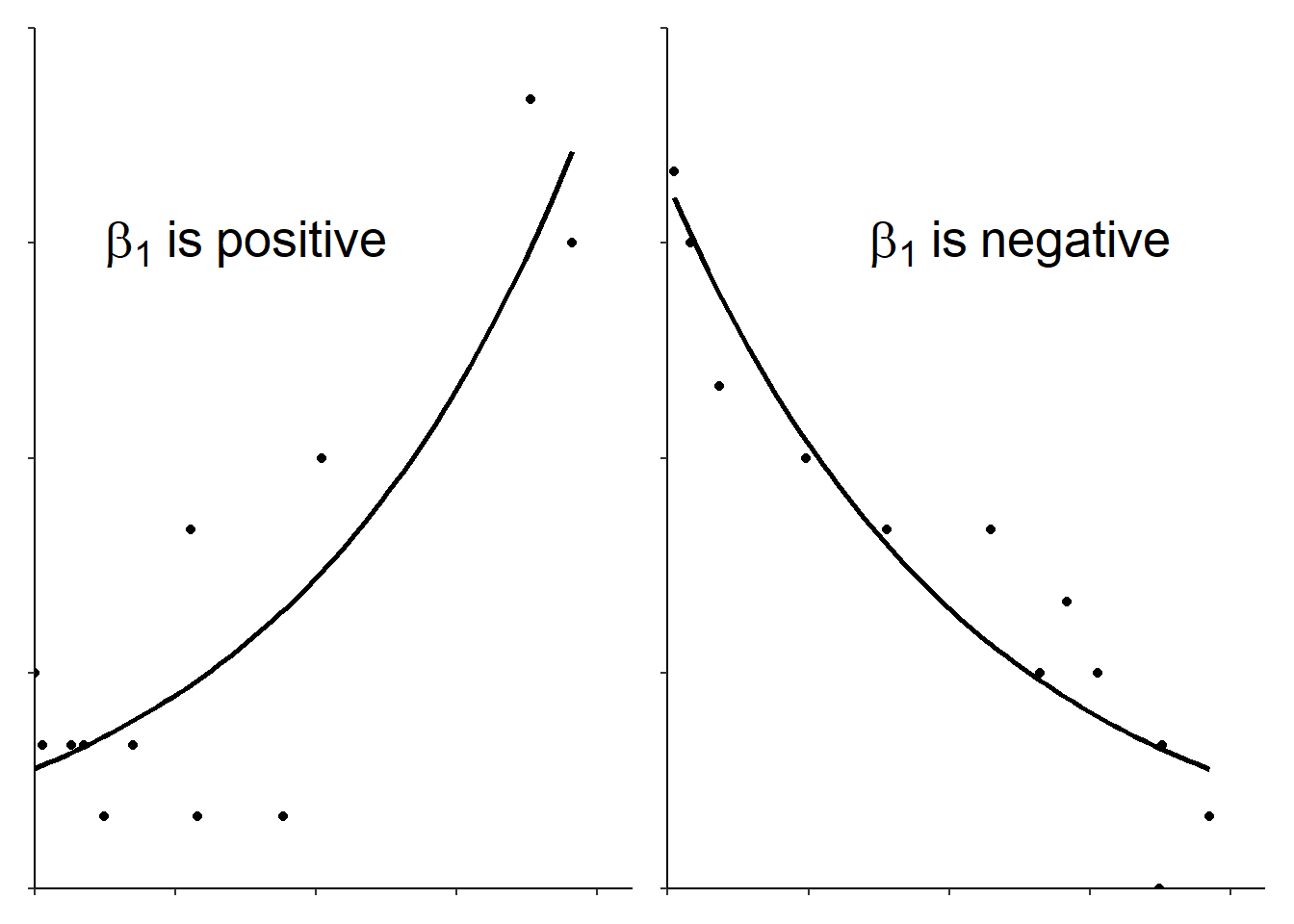
Just like examples of general linear models with a single explanatory variable, there are two parameters in this model, \(\beta_{0}\) and \(\beta_{0}\) and their meaning is similar. \(\beta_{0}\) is the log of the expected \(y\) when \(x\) is zero (i.e., the intercept). The log of \(\beta_{1}\) is not the amount you add to \(y\) for each unit change in \(x\) but the amount by which to multiply. This means the model is a curve. If \(\beta_{1}\) is positive, \(exp(\beta_{1})\) is greater than one and \(y\) increases as \(x\) increases; if \(\beta_{1}\) is negative, \(exp(\beta_{1})\) is less than one and \(y\) decreases as \(x\) increases. See Figure 2.1 for an illustration of the curve for positive and negative \(\beta_{1}\).

Figure 2.1: Data fitted with a Poisson GLM.
See Figure 2.2 for a graphical representation of generalised linear model terms.
Figure 2.2: A Generalised linear model with Poisson distributed errors. The measured response values are in pink, the predictions are in green, and the differences between these, known as the residuals, are in blue. The estimated model parameters, \(\beta_{0}\) and \(\beta_{1}\) must be exponentiated to be interpreted on the scale of the response. When \(x=0\) we predict the number of \(y\) to be \(exp(\beta_{0})\). For each unit of \(x\), the number of \(y\) changes by a factor of \(exp(\beta_{1})\)
\(ln\) is the link function in a Poisson GLM. The estimates are log counts and using \(exp(\beta_{0})\) and \(exp(\beta_{1})\) enables us to interpret them as counts.
2.1 When explanatory is categorical
If your response is a count and you just one categorical explanatory variable you do not need a Poisson GLMS. Use a chi-squared test.
2.2 More than one explanatory
\[\begin{equation} ln(E(y_{i}))=\beta_{0}+\beta_{1}X1_{i}+\beta_{2}X2_{i}+...+\beta_{p}Xp_{i} \tag{2.4} \end{equation}\]
To make predictions about the expected value of the response we need to exponentiate the coefficients.
\[\begin{equation} E(y_{i})=exp(\beta_{0}+\beta_{1}X1_{i}+\beta_{2}X2_{i}+...+\beta_{p}Xp_{i}) \tag{2.5} \end{equation}\]
2.3 Reporting
The important information to include when reporting the results of fitting a Poisson GLM are the most notable predictions and the significance, direction and magnitude of effects. You need to ensure your reader will understand what the data are saying even if all the numbers and statistical information was removed. For example, variable \(Y\) increases with variables \(X1\).
In relatively simple models, reporting group means or a slope, and statistical test information is enough. In more complex models with many variables is it common to give all the estimated model coefficients in a table.
In addition, your figure should show both the data and the model. This is honest and allows your interpretation to be evaluated.