3 Single continuous explanatory
3.1 Introduction to the example
The number of cases of cancer reported by a clinic and its distance, in kilometres, from a nuclear plant were recorded and the data are in cases.txt. Researchers wanted to know if proximity to the nuclear power plant influenced the incidence of cancer. Bear in mind this is not great epidemiology - there would be very many other factors influencing the occurrence and reporting of cancer cases at a clinic.
| cancers | distance |
|---|---|
| 0 | 154.37 |
| 0 | 93.14 |
| 4 | 3.83 |
| 0 | 60.83 |
| 0 | 142.61 |
| 0 | 164.72 |
| 0 | 135.92 |
| 1 | 79.92 |
| 0 | 112.71 |
| 0 | 101.76 |
| 2 | 59.62 |
| 0 | 128.07 |
| 2 | 17.17 |
| 1 | 24.81 |
| 1 | 103.42 |
| 0 | 112.70 |
| 0 | 143.96 |
| 1 | 48.77 |
| 1 | 82.20 |
| 1 | 57.53 |
| 1 | 12.75 |
| 0 | 64.47 |
| 1 | 68.78 |
| 1 | 133.40 |
| 0 | 98.94 |
| 0 | 40.87 |
| 0 | 151.82 |
| 4 | 35.15 |
| 0 | 97.10 |
| 0 | 131.44 |
| 0 | 102.02 |
| 0 | 116.77 |
| 1 | 28.79 |
| 0 | 52.63 |
| 2 | 23.15 |
| 1 | 68.13 |
| 0 | 146.93 |
| 1 | 87.98 |
| 0 | 147.30 |
| 1 | 132.67 |
| 0 | 164.21 |
| 1 | 72.67 |
| 0 | 22.81 |
There are 2 variables: the response, cancers, is the number of cancer cases reported at a clinic and distance, gives the clinic’s distance from the nuclear plant.
We will import the data with the read_table() function and plot it with ggplot().
cases <- read_table("data-raw/cases.txt")
# a default scatter plot of the data
ggplot(data = cases, aes(x = distance, y = cancers)) +
  geom_point()
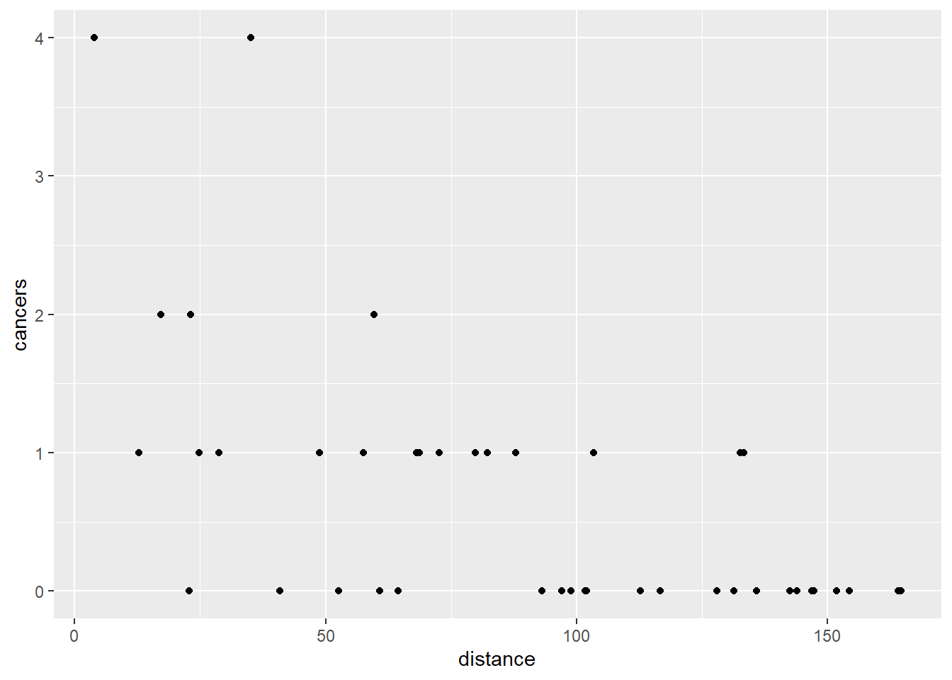
Most of the clinics reporting no cases seem to be more distance from the nuclear plant and those reporting the highest numbers are within 50km.
3.2 Applying and interpreting glm()
We build a generalised linear model of the number of cases explained by the distance with the glm() function as follows:
mod <- glm(data = cases, cancers ~ distance, family = poisson)Printing mod to the console gives us the estimated model parameters:
mod
#
# Call:  glm(formula = cancers ~ distance, family = poisson, data = cases)
#
# Coefficients:
# (Intercept)     distance
#      1.0192      -0.0215
#
# Degrees of Freedom: 42 Total (i.e. Null);  41 Residual
# Null Deviance:        54.5
# Residual Deviance: 31.8   AIC: 78.2
We will postpone discussing the information in the last three lines until we view the model summary.
\(\beta_{0}\) is labelled “(Intercept)” and \(\beta_{1}\) is labelled “distance.” Thus the equation of the line is:
The fact that the estimate for distance (-0.021) is negative tells us that as distance increases, the number of cancers reported goes down.
These estimates are on the scale of the link function, that is, they are logged (to the base e, natural logs) in this case.
To understand the parameters the on the scale of the response we apply the inverse of the \(ln\) function, the exp() function
exp(mod$coefficients)
# (Intercept)    distance
# 2.771 0.979The model predicts there will be 2.771 cancers at a clinic at 0 km from the power plant.
Recall that for a linear model with one predictor, the second estimate is the amount added to the intercept when the predictor changes by one value. Since this is GLM with a log link, the value of 0.979 is amount the intercept is multiplied by for each unit increase of distance. Thus the model predicts there will be 2.771 \(\times\) 0.979 = 2.712 cancers 1 km away and 2.771 \(\times\) 0.979 \(\times\) 0.979 = 2.654 cancers 2 km away. That is: \(\beta_{0}\) \(\times\) \(\beta_{0}^n\) mm at \(n\) km away.
You can work these out either by exponentiating the coefficients and then multiplying the results or by adding the coefficients and exponentiating.
Exponentiate coefficients then multiply:
# 1km away
exp(b0) * exp(b1)
# [1] 2.71

# 2km away
exp(b0) * exp(b1) * exp(b1)
# [1] 2.65

# 10km away
exp(b0) * exp(b1)^10
# [1] 2.23
Add the coefficients then exponentiate the sum:
# 1km away
exp(b0 + b1)
# [1] 2.71

# 2km away
exp(b0 + b1 + b1)
# [1] 2.65

# 10km away
exp(b0 + 10*b1)
# [1] 2.23
The model predicts the number of cancers at 0 km from the plant will be 2.771, which is \(exp(\beta_{0})\). This decreases by a factor of 0.979 for each km away which is \(exp(\beta_{1})\). This something you multiply by rather than add because the link function is a log.
Usually, we use the predict() function to make predictions for particular distances (see later).
More information including statistical tests of the model and its parameters is obtained by using summary():
summary(mod)
#
# Call:
# glm(formula = cancers ~ distance, family = poisson, data = cases)
#
# Deviance Residuals:
#    Min      1Q  Median      3Q     Max
# -1.842  -0.744  -0.483   0.421   1.893
#
# Coefficients:
#             Estimate Std. Error z value Pr(>|z|)
# (Intercept)  1.01917    0.30871    3.30  0.00096 ***
# distance    -0.02150    0.00503   -4.27  0.00002 ***
# ---
# Signif. codes:  0 '***' 0.001 '**' 0.01 '*' 0.05 '.' 0.1 ' ' 1
#
# (Dispersion parameter for poisson family taken to be 1)
#
#     Null deviance: 54.522  on 42  degrees of freedom
# Residual deviance: 31.790  on 41  degrees of freedom
# AIC: 78.16
#
# Number of Fisher Scoring iterations: 5
The Coefficients table gives the estimated \(\beta_{0}\) and \(\beta_{1}\) again but along with their standard errors and tests of whether the estimates differ from zero. The estimated value for the intercept is 1.019 \(\pm\) 0.309 and this differs significantly from zero (\(p\) < 0.001). The estimated value for the slope is -0.021 \(\pm\) 0.005, also differs significantly from zero (\(p\) < 0.001).
Towards the bottom of the output there is information about the model fit. The null deviance (what exists if we predict the number of cases from an intercept, \(\beta_{0}\), only model) is 54.522 with 42 degrees of freedom and the residual deviance (left over after our model is fitted) is 31.79 with 41 \(d.f.\). The model fits a 1 parameter, \(\beta_{1}\), and thus accounts for 1 \(d.f.\) for a reduction in deviance by 22.732.
To get a test of whether the reduction in deviance is significant for each term in the the model formula we use:
To get a test of the model overall:
anova(mod, test = "Chisq")
# Analysis of Deviance Table
#
# Model: poisson, link: log
#
# Response: cancers
#
# Terms added sequentially (first to last)
#
#
#          Df Deviance Resid. Df Resid. Dev  Pr(>Chi)
# NULL                        42       54.5
# distance  1     22.7        41       31.8 0.0000019 ***
# ---
# Signif. codes:  0 '***' 0.001 '**' 0.01 '*' 0.05 '.' 0.1 ' ' 1
There is a significant reduction in deviance for our model (p < 0.001). Note that there is only one term in this model.
The number of cancers decreases significantly with distance
3.3 Getting predictions from the model
The predict() function returns the predicted values of the response. To add a column of predicted values to the dataframe:
we need to specify they should be on the scale of the responses, not on the link function scale.
cases$pred <- predict(mod, type = "response")This gives predictions for the actual \(x\) values used. If you want predicts for other values of \(x\) you need to create a data frame of the \(x\) values from which you want to predict
For example, to predict for distances from 0 to 180 km in steps of 10 km:
predict_for <- data.frame(distance = seq(0, 180, 10))
predict_for$pred <- predict(mod, newdata = predict_for, type = "response")3.4 Creating a figure
ggplot(data = cases, aes(x = distance, y = cancers)) +
  geom_point() +
geom_smooth(method = "glm",
              method.args = list(family = "poisson"),
              se = FALSE,
            colour = "black") +
  scale_x_continuous(expand = c(0, 0),
                     limits = c(0, 190),
                     name = "Distance (km) of clinic from plant") +
    scale_y_continuous(expand = c(0, 0.03),
                     limits = c(0, 5),
                     name = "Number of reported cancers") +
  theme_classic()

3.5 Reporting the results
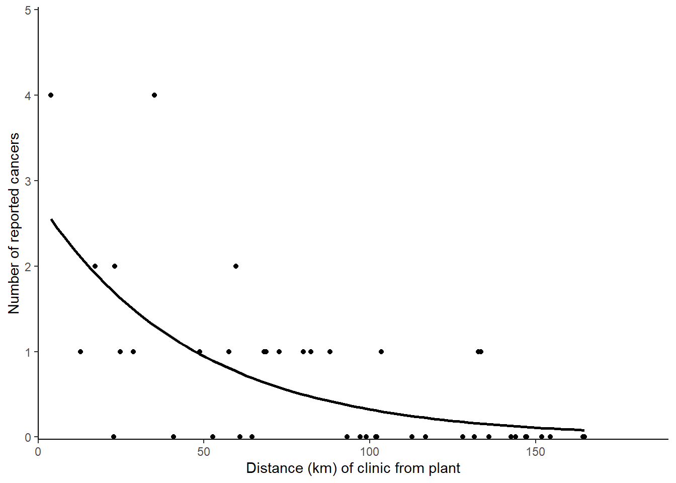
The number of cases reported by a clinic significantly decreases by a factor of 0.979 \(\pm\) 1.005 for each kilometre from the nuclear plant (p < 0.001). See figure 3.1. For a clinic at the plant, 2.771 \(\pm\) 1.362 cases are expected

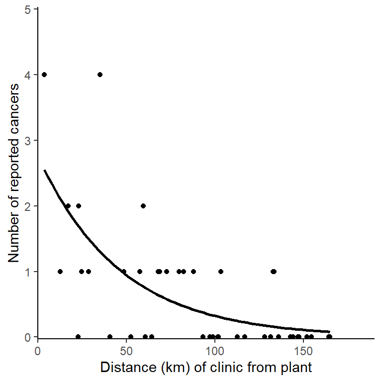
Figure 3.1: Incidence of cancer cases reported at clinic by it distance from the nuclear plant. The line gives predictions for a GLM with Poisson distributed errors, \(y\) = 2.771 \(\times\) 0.979\(^{x}\).