Workshop

One-way ANOVA and Kruskal-Wallis

Introduction

Artwork by Horst (2023): “Debugging and feelings”

Session overview

In this session you will get practice in choosing between, performing, and presenting the results of, one-way ANOVA and Kruskal-Wallis in R.

Philosophy

Workshops are not a test. It is expected that you often don’t know how to start, make a lot of mistakes and need help. It is expected that you are familiar with independent study content before the workshop. However, you need not remember or understand every detail as the workshop should build and consolidate your understanding. Tips

don’t worry about making mistakes
don’t let what you can not do interfere with what you can do
discussing code with your neighbours will help
look things up in the independent study material
look things up in your own code from earlier
there are no stupid questions

Key

These four symbols are used at the beginning of each instruction so you know where to carry out the instruction.

Something you need to do on your computer. It may be opening programs or documents or locating a file.

Something you should do in RStudio. It will often be typing a command or using the menus but might also be creating folders, locating or moving files.

Something you should do in your browser on the internet. It may be searching for information, going to the VLE or downloading a file.

A question for you to think about and answer. Record your answers in your script for future reference.

Getting started

Start RStudio from the Start menu.

Go the Files tab in the lower right pane and click on the ... on the right. This will open a “Go to folder” window. Navigate to a place on your computer where you keep your work. Click Open.

Make an RStudio project for this workshop by clicking on the drop-down menu on top right where it says Project: (None) and choosing New Project, then New Directory, then New Project. Navigate to the data-analysis-in-r-2 folder and name the RStudio Project week-4.

Make new folders called data-raw and figures. You can do this on the Files Pane by clicking New Folder and typing into the box that appears.

Make a new script then save it with a name like one-way-anova-and-kw.R to carry out the rest of the work.

Add a comment to the script: # One-way ANOVA and Kruskal-Wallis and load the tidyverse (Wickham et al. 2019) package

Exercises

Myoglobin in seal muscle

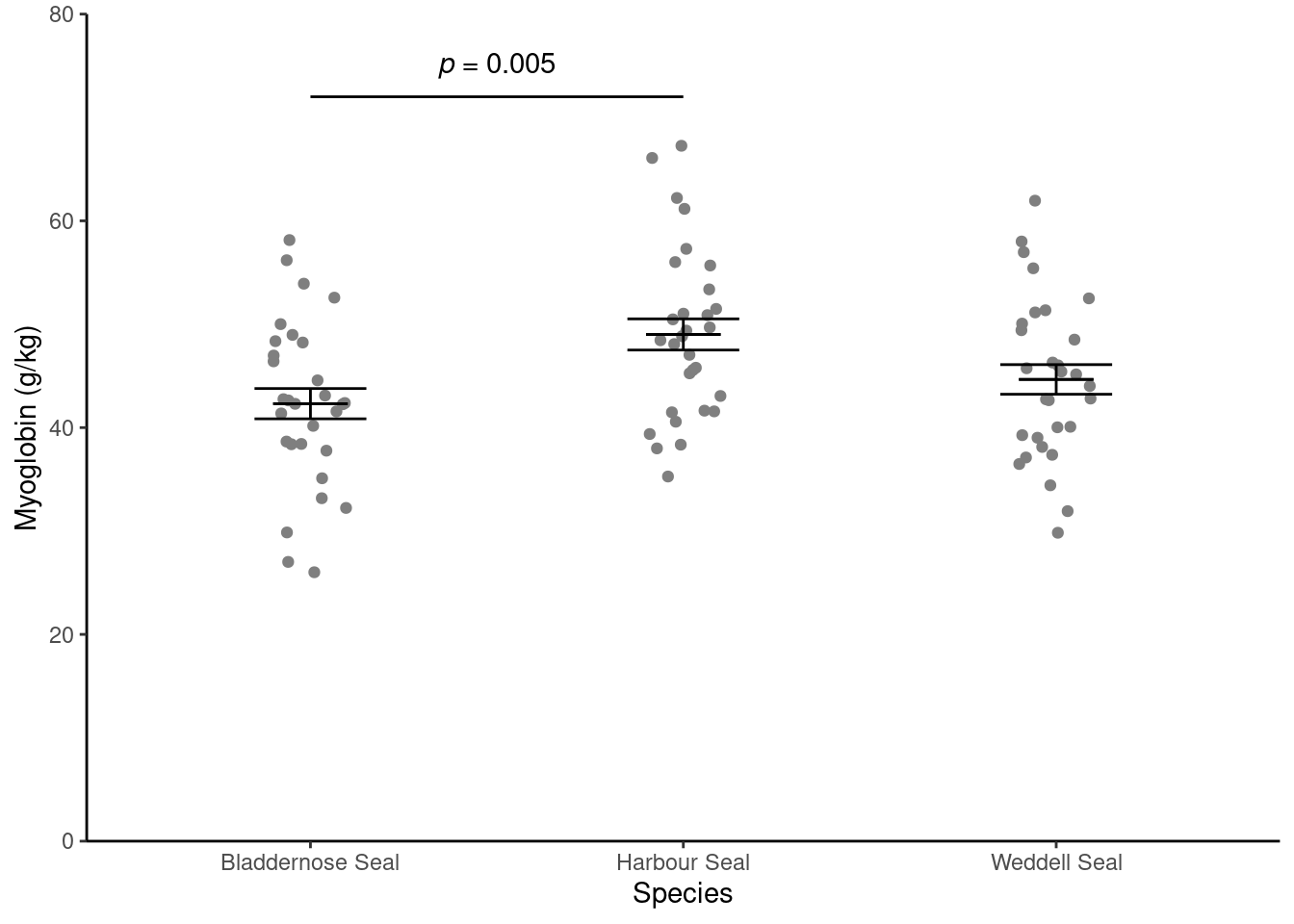
The myoglobin concentration of skeletal muscle of three species of seal in grams per kilogram of muscle was determined and the data are given in seal.csv. We want to know if there is a difference between species. Each row represents an individual seal. The first column gives the myoglobin concentration and the second column indicates species.

Save a copy of the data file seal.csv to data-raw

Read in the data and check the structure. I used the name seal for the dataframe/tibble.

What kind of variables do you have?

Exploring

Do a quick plot of the data. You may need to refer to a previous workshop

Summarising the data

Do you remember Look after future you!

If you followed that tip you’ll be able to open that script and whizz through summarising,testing and plotting.

Create a data frame called seal_summary that contains the means, standard deviations, sample sizes and standard errors for each species.

You should get the following numbers:

species	mean	std	n	se
Bladdernose Seal	42.31600	8.020634	30	1.464361
Harbour Seal	49.01033	8.252004	30	1.506603
Weddell Seal	44.66033	7.849816	30	1.433174

Applying, interpreting and reporting

We can now carry out a one-way ANOVA using the same lm() function we used for two-sample tests.

Carry out an ANOVA and examine the results with:

mod <- lm(data = seal, myoglobin ~ species)
summary(mod)


Call:
lm(formula = myoglobin ~ species, data = seal)

Residuals:
    Min      1Q  Median      3Q     Max 
-16.306  -5.578  -0.036   5.240  18.250 

Coefficients:
                    Estimate Std. Error t value Pr(>|t|)    
(Intercept)           42.316      1.468  28.819  < 2e-16 ***
speciesHarbour Seal    6.694      2.077   3.224  0.00178 ** 
speciesWeddell Seal    2.344      2.077   1.129  0.26202    
---
Signif. codes:  0 '***' 0.001 '**' 0.01 '*' 0.05 '.' 0.1 ' ' 1

Residual standard error: 8.043 on 87 degrees of freedom
Multiple R-squared:  0.1096,    Adjusted R-squared:  0.08908 
F-statistic: 5.352 on 2 and 87 DF,  p-value: 0.006427

Remember: the tilde (~) means test the values in myoglobin when grouped by the values in species. Or explain myoglobin with species

What do you conclude so far from the test? Write your conclusion in a form suitable for a report.

Can you relate the values under Estimate to the means?

The ANOVA is significant but this only tells us that species matters, meaning at least two of the means differ. To find out which means differ, we need a post-hoc test. A post-hoc (“after this”) test is done after a significant ANOVA test. There are several possible post-hoc tests and we will be using Tukey’s HSD (honestly significant difference) test (Tukey 1949) implemented in the emmeans (Lenth 2023) package.

Load the package

library(emmeans)

Carry out the post-hoc test

emmeans(mod, ~ species) |> pairs()

 contrast                        estimate   SE df t.ratio p.value
 Bladdernose Seal - Harbour Seal    -6.69 2.08 87  -3.224  0.0050
 Bladdernose Seal - Weddell Seal    -2.34 2.08 87  -1.129  0.4990
 Harbour Seal - Weddell Seal         4.35 2.08 87   2.095  0.0968

P value adjustment: tukey method for comparing a family of 3 estimates

Each row is a comparison between the two means in the ‘contrast’ column. The ‘estimate’ column is the difference between those means and the ‘p.value’ indicates whether that difference is significant.

A plot can be used to visualise the result of the post-hoc which can be especially useful when there are very many comparisons.

Plot the results of the post-hoc test:

emmeans(mod, ~ species) |> plot()

Where the purple bars overlap, there is no significant difference.

What do you conclude from the test?

Check assumptions

The assumptions of the general linear model are that the residuals – the difference between predicted value (i.e., the group mean) and observed values - are normally distributed and have homogeneous variance. To check these we can examine the mod$residuals variable. You may want to refer to Checking assumptions in the “Single regression” workshop.

Plot the model residuals against the fitted values.

What to you conclude?

To examine normality of the model residuals we can plot them as a histogram and do a normality test on them.

Plot a histogram of the residuals.

Use the shapiro.test() to test the normality of the model residuals

What to you conclude?

Illustrating

Create a figure like the one below. You may need to refer to Visualise from the “Summarising data with several variables” workshop (Rand 2023)

We will again use both our seal and seal_summary dataframes.

Create the plot:

Save your figure to your figures folder.

Leafminers on Birch

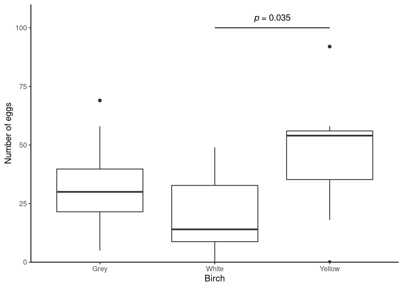
Larvae of the Ambermarked birch leafminer, Profenusa thomsoni, feed on the interior leaf tissues of Birch (Betula) species. They do not normally kill the tree but can weaken it making it susceptible to attack from other species. Researchers are interested in whether there is a difference in the rates at which white, grey and yellow birch are attacked. They introduce adult female P.thomsoni to a green house containing 30 young trees (ten of each type) and later count the egg laying events on each tree. The data are in leaf.txt.

Exploring

Read in the data and check the structure. I used the name leaf for the dataframe/tibble.

What kind of variables do we have?

Do a quick plot of the data.

Using your common sense, do these data look normally distributed?

Why is a Kruskal-Wallis appropriate in this case?

Calculate the medians, means and sample sizes.

Applying, interpreting and reporting

Carry out a Kruskal-Wallis:

kruskal.test(data = leaf, eggs ~ birch)


    Kruskal-Wallis rank sum test

data:  eggs by birch
Kruskal-Wallis chi-squared = 6.3393, df = 2, p-value = 0.04202

What do you conclude from the test?

A significant Kruskal-Wallis tells us at least two of the groups differ but where do the differences lie? The Dunn test is a post-hoc multiple comparison test for a significant Kruskal-Wallis. It is available in the package FSA

Load the package using:

library(FSA)

Run the post-hoc test with:

dunnTest(data = leaf, eggs ~ birch)

      Comparison         Z    P.unadj      P.adj
1   Grey - White  1.296845 0.19468465 0.38936930
2  Grey - Yellow -1.220560 0.22225279 0.22225279
3 White - Yellow -2.517404 0.01182231 0.03546692

The P.adj column gives p-value for the comparison listed in the first column. Z is the test statistic.

What do you conclude from the test?

Write up the result is a form suitable for a report.

Illustrating

A box plot is an appropriate choice for illustrating a Kruskal-Wallis. Can you produce a figure like this?

You’re finished!

🥳 Well Done! 🎉

Illustrations from the Openscapes blog Tidy Data for reproducibility, efficiency, and collaboration by Julia Lowndes and Allison Horst

Independent study following the workshop

Consolidate

The Code file

This contains all the code needed in the workshop even where it is not visible on the webpage.

The workshop.qmd file is the file I use to compile the practical. Qmd stands for Quarto markdown. It allows code and ordinary text to be interweaved to produce well-formatted reports including webpages. View the Qmd in Browser. Coding and thinking answers are marked with #---CODING ANSWER--- and #---THINKING ANSWER---

Pages made with R (R Core Team 2023), Quarto (Allaire et al. 2022), knitr (Xie 2022), kableExtra (Zhu 2021)

References

Allaire, J. J., Charles Teague, Carlos Scheidegger, Yihui Xie, and Christophe Dervieux. 2022. Quarto. https://doi.org/10.5281/zenodo.5960048.

Horst, Allison. 2023. “Data Science Illustrations.” https://allisonhorst.com/allison-horst.

Lenth, Russell V. 2023. Emmeans: Estimated Marginal Means, Aka Least-Squares Means. https://CRAN.R-project.org/package=emmeans.

R Core Team. 2023. R: A Language and Environment for Statistical Computing. Vienna, Austria: R Foundation for Statistical Computing. https://www.R-project.org/.

Rand, Emma. 2023. Data Analysis in r for Becoming a Bioscientist. https://3mmarand.github.io/R4BABS/.

Tukey, John W. 1949. “Comparing Individual Means in the Analysis of Variance.” Biometrics 5 (2): 99–114. https://doi.org/10.2307/3001913.

Wickham, Hadley, Mara Averick, Jennifer Bryan, Winston Chang, Lucy D’Agostino McGowan, Romain François, Garrett Grolemund, et al. 2019. “Welcome to the Tidyverse” 4: 1686. https://doi.org/10.21105/joss.01686.

Xie, Yihui. 2022. “Knitr: A General-Purpose Package for Dynamic Report Generation in r.” https://yihui.org/knitr/.

Zhu, Hao. 2021. “kableExtra: Construct Complex Table with ’Kable’ and Pipe Syntax.” https://CRAN.R-project.org/package=kableExtra.