Workshop

Association: Correlation and Contingency

Introduction

Animated gif of the R logo with a rainbow that grows over the logo repeatedly.

Artwork by Horst (2023):

Session overview

In this session you will:

test whether there is an association two continuous variables using parametric and non-parametric correlations
learn about the effect of sample size on correlation
test whether there is an association between two categorical variables using the chi-squared contingency test

Philosophy

Workshops are not a test. It is expected that you often don’t know how to start, make a lot of mistakes and need help. It is expected that you are familiar with independent study content before the workshop. However, you need not remember or understand every detail as the workshop should build and consolidate your understanding. Tips

don’t worry about making mistakes
don’t let what you can not do interfere with what you can do
discussing code with your neighbours will help
look things up in the independent study material
look things up in your own code from earlier
there are no stupid questions

Key

These four symbols are used at the beginning of each instruction so you know where to carry out the instruction.

Something you need to do on your computer. It may be opening programs or documents or locating a file.

Something you should do in RStudio. It will often be typing a command or using the menus but might also be creating folders, locating or moving files.

Something you should do in your browser on the internet. It may be searching for information, going to the VLE or downloading a file.

A question for you to think about and answer. Record your answers in your script for future reference.

Getting started

Start RStudio from the Start menu.

Make an RStudio project for this workshop by clicking on the drop-down menu on top right where it says Project: (None) and choosing New Project, then New Directory, then New Project. Navigate to the data-analysis-in-r-2 folder and name the RStudio Project week-6.

Make new folders called data-raw and figures. You can do this on the Files Pane by clicking New Folder and typing into the box that appears.

Make a two new scripts called correlation.R and contingency-chi-squared-tests.R to carry out the rest of the work.

Add a comments to each script such as: # Correlation and # Contingency Chi-squared tests and load the tidyverse (Wickham et al. 2019) package in each

Exercises

Pearson’s Correlation

The data given in height.txt are the heights of eleven sibling pairs.

Save a copy of height.txt to your data-raw folder and import it.

Top Tip

Did you know you can also read a file directly from the internet instead of saving it first?

height <- read_table("https://3mmarand.github.io/R4BABS/r4babs2/week-6/data-raw/height.txt")

This valuable if you need the latest version of a regularly updated file.

However, if you are concerned about the file disappearing or moving, then it would be better to save it.

Exploring

What type of variables are older and younger? What are the implications for the test?

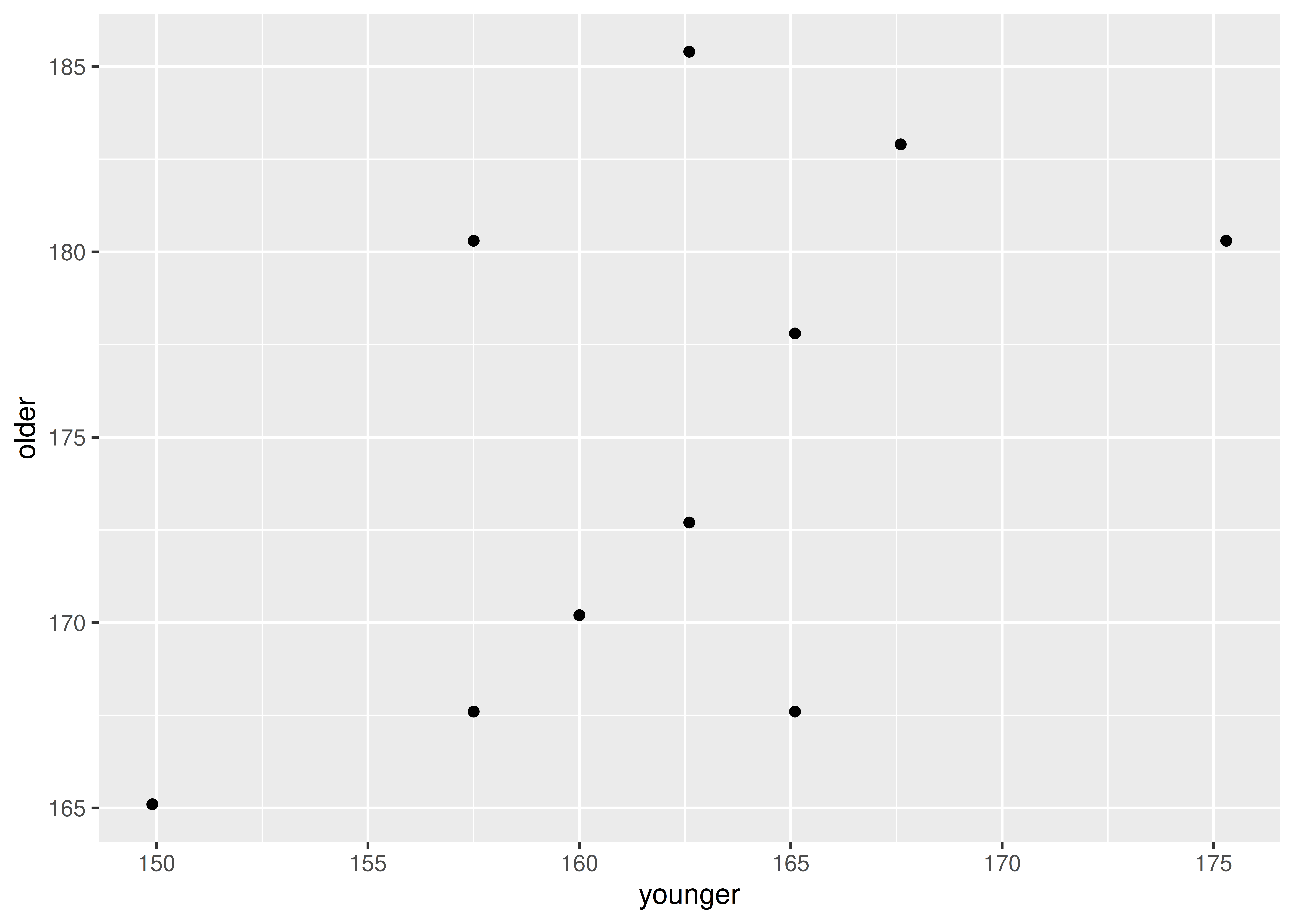
Do a quick plot of the data. We don’t have a causal relationship here so either variable can go on the x-axis.

ggplot(height, aes(x = younger, y = older) ) +
  geom_point()

Remembering that one of the assumptions for parametric correlation is that any correlation should be linear, what do you conclude from the plot?

Applying, interpreting and reporting

We will do a parametric correlation.

We can carry out a Pearson’s product moment correlation with:

cor.test(data = height, ~ older + younger, method = "pearson")


    Pearson's product-moment correlation

data:  older and younger
t = 2.0157, df = 9, p-value = 0.07464
alternative hypothesis: true correlation is not equal to 0
95 percent confidence interval:
 -0.06336505  0.86739285
sample estimates:
      cor 
0.5577091

Notice:

we are not using the response ~ explanatory form here because this is not a causal relationship.
Pearson is the default correlation method, therefore we could omit method = "pearson".

What do you conclude from the test?

Illustrating

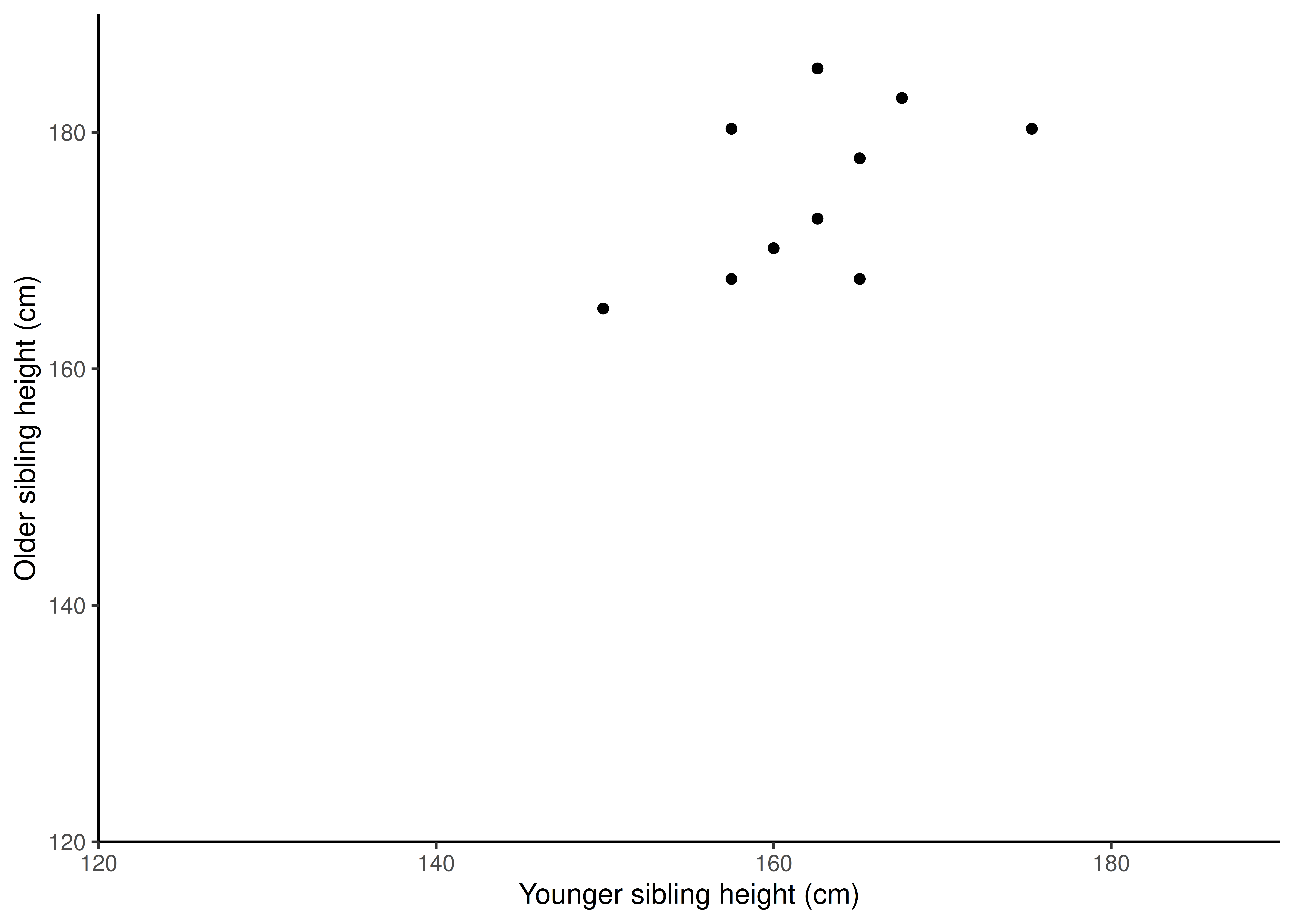
Create a better figure for our data using:

fig1 <- ggplot(height, aes(x = younger, y = older)) +
  geom_point() +
  scale_x_continuous(name = "Younger sibling height (cm)",
                     limits = c(120, 190),
                     expand = c(0, 0)) +
  scale_y_continuous(name = "Older sibling height (cm)",
                     limits = c(120, 190),
                     expand = c(0, 0)) +
   theme_classic()

fig1

Figure legend - Axes

In this figure we have started the axes at 120 so we can see the data more easily. You would want to draw the readers attention to this in the figure legend.

Use ggsave() to save your figure to file in your figures folder.

Effect of sample size on correlation

Now we will explore the effect of sample size on the value of the correlation coefficient and its significance.

Create a dataset with twice the number of observations:

height2 <- rbind(height, height)

rbind() binds rows together so it repeats the data. Make sure you view the resulting dataframe. Each pair of values will appear twice.

Now repeat the correlation with height2

What do you conclude? What does this tell you about the sensitivity of correlation to sample size?

Spearman’s rank Correlation

Since our sibling dataset is so small we might very reasonably have chosen to do a non-parametric correlation on the grounds that it is difficult to determine either normality or linearity on small samples.

The same function is used for a non-parametric correlation but we specify a different value for the method argument.

Carry out a Spearman’s rank correlation:

cor.test(data = height, ~ older + younger, method = "spearman")


    Spearman's rank correlation rho

data:  older and younger
S = 109.74, p-value = 0.1163
alternative hypothesis: true rho is not equal to 0
sample estimates:
      rho 
0.5011722

What do you conclude?

Contingency chi-squared test

A human geneticist found that in a sample of 477 blood group O people 65 had peptic ulcers whereas in a sample of 387 blood group A people 31 had peptic ulcers.

Draw a 2 x 2 table of these data (on a piece of paper).

What is your null hypothesis?

Make a vector obs that holds the 4 observed numbers. For the moment, don’t worry about what order they are in.

Completely forgotten how to make a vector?

Since we have been reading date in from files, you might have forgotten how to create a vector of values. You can remind yourself from either:

Computational Analysis for Bioscientists: To create a vector called ages of several numbers
BABS 1 Week 7 Workshop (our first): Making vector that hold cat coat colours

You have used vectors a lot since - every time you have used c(....) - but you might not have realised it.

For a contingency chi squared test, the inbuilt chi-squared test can be used in a straightforward way. However, we need to structure our data as a 2 x 2 table rather than as a 1 x 4 vector. A 2 x 2 table can be created with the matrix() function. We can also name the rows and columns which helps us interpret the results.

To create a list containing two elements which are vectors for the two groups in each variable we do:

# list of two elements
# the two variables are whether someone has an ulcer or not and whether 
# they are blood group O or A
vars <- list(ulcer = c("yes","no"), blood = c("O", "A"))
vars

$ulcer
[1] "yes" "no" 

$blood
[1] "O" "A"

Now we can create the matrix from our vector of numbers obs and use our list vars to give the column and row names:

ulcers <- matrix(obs, nrow = 2, dimnames = vars)
ulcers

     blood
ulcer   O   A
  yes  65  31
  no  412 356

Check the content of ulcers and recreate if the numbers are not in the correct place (i.e., do not match your table)

Run a contingency chi-squared with:

chisq.test(ulcers, correct = FALSE)


    Pearson's Chi-squared test

data:  ulcers
X-squared = 6.824, df = 1, p-value = 0.008994

This significant ($p = $ 0.009) so we know that the proportion of people with an ulcer is different in the two blood groups. In other words, there is an association between ulcers and blood group.

It is not obvious from the printed test information, which blood group has a higher association with ulcers. We can find this out by examining the expected values were. The expected values are what we expect to see if the null hypothesis is correct. They can be accessed in the $expected variable in the output value of the chisq.test() method (See the manual!).

View the expected values with:

chisq.test(ulcers, correct = FALSE)$expected

     blood
ulcer   O   A
  yes  53  43
  no  424 344

What do you conclude about the association between ABO blood group and peptic ulcers?

Blood group and ulcers- alternative data format.

The data you have just used were already tabulated. Often data arrives untabluated - imagine you have several medical variables about individuals, you would have an invidual in each row with columns indicating blood group and ulcer status along with other measures such as age, height and mass.

There are raw data in blood_ulcers.txt. Examine this file to understand the format

Save a copy of blood_ulcers.txt to your data-raw folder

Read the data in to R and check the structure.

We can tabulate the data and assign it using the table() command:

ulctab <- table(blood_ulcers$blood, blood_ulcers$ulcer)
# examine the result
ulctab

We need to give both variables to cross tabulate.

Now carry out the contingency chi-squared like this:

chisq.test(ulctab, correct = FALSE)


    Pearson's Chi-squared test

data:  ulctab
X-squared = 6.824, df = 1, p-value = 0.008994

Congratulations on making it to the end of the stage 1 Data Analysis in R teaching!

Animated gif with pastel lines in the background. The words 'CODE HERO' in bold black text scroll across repeatedly. — Artwork by Horst (2023):

Independent study following the workshop

Consolidate

The Code file

This contains all the code needed in the workshop even where it is not visible on the webpage.

The workshop.qmd file is the file I use to compile the practical. Qmd stands for Quarto markdown. It allows code and ordinary text to be interweaved to produce well-formatted reports including webpages. View the Qmd in Browser. Coding and thinking answers are marked with #---CODING ANSWER--- and #---THINKING ANSWER---

Pages made with R (R Core Team 2024), Quarto (Allaire et al. 2022), knitr (Xie 2024, 2015, 2014), kableExtra (Zhu 2024)

References

Allaire, J. J., Charles Teague, Carlos Scheidegger, Yihui Xie, and Christophe Dervieux. 2022. Quarto. https://doi.org/10.5281/zenodo.5960048.

Horst, Allison. 2023. “Data Science Illustrations.” https://allisonhorst.com/allison-horst.

R Core Team. 2024. R: A Language and Environment for Statistical Computing. Vienna, Austria: R Foundation for Statistical Computing. https://www.R-project.org/.

Wickham, Hadley, Mara Averick, Jennifer Bryan, Winston Chang, Lucy D’Agostino McGowan, Romain François, Garrett Grolemund, et al. 2019. “Welcome to the Tidyverse” 4: 1686. https://doi.org/10.21105/joss.01686.

Xie, Yihui. 2014. “Knitr: A Comprehensive Tool for Reproducible Research in R.” In Implementing Reproducible Computational Research, edited by Victoria Stodden, Friedrich Leisch, and Roger D. Peng. Chapman; Hall/CRC.

———. 2015. Dynamic Documents with R and Knitr. 2nd ed. Boca Raton, Florida: Chapman; Hall/CRC. https://yihui.org/knitr/.

———. 2024. Knitr: A General-Purpose Package for Dynamic Report Generation in r. https://yihui.org/knitr/.

Zhu, Hao. 2024. kableExtra: Construct Complex Table with ’Kable’ and Pipe Syntax. https://CRAN.R-project.org/package=kableExtra.