7  First Steps in RStudio

First draft

You are reading a work in progress. This page is a first draft but should be readable.

This chapter …..

Right, let’s start coding!

7.0.1 Your first piece of code

We can use R just like a calculator. Put your cursor after the > in the Console, type 3 + 4 and ↵ Enter to send that command:

3+4
## [1] 7

The > is called the “prompt”. You do not have to type it, it tells you that R is ready for input.

Where I’ve written 3+4, I have no spaces. However, you can have spaces, and in fact, it’s good practice to use spaces around your operators because it makes your code easier to read. So a better way of writing this would be:

3 + 4
## [1] 7

In the output we have the number 7, which, obviously, is the answer. From now on, you should assume commands typed at the console should be followed by ↵ Enter to send them.

The one in parentheses, [1], is an index. It is telling you that the 7 is the first element of the output. We can see this more clear if we create something with more output. For example, 50:100 will print the numbers from 50 to 100.

50:100
##  [1]  50  51  52  53  54  55  56  57  58  59  60  61  62  63  64  65  66  67  68
## [20]  69  70  71  72  73  74  75  76  77  78  79  80  81  82  83  84  85  86  87
## [39]  88  89  90  91  92  93  94  95  96  97  98  99 100

The numbers in the square parentheses at the beginning of the line give you the index of the first element in the line. R is telling you where you are in the output.

7.0.2 Assigning variables

Very often we want to keep input values or output for future use. We do this with ‘assignment’ An assignment is a statement in programming that is used to set a value to a variable name. In R, the operator used to do assignment is <-. It assigns the value on the right-hand to the value on the left-hand side.

To assign the value 3 to x we do:

x <- 3

and ↵ Enter to send that command.

The assignment operator is made of two characters, the < and the - and there is a keyboard short cut: Alt+- (windows) or Option+- (Mac). Using the shortcut means you’ll automatically get spaces. You won’t see any output when the command has been executed because there is no output. However, you will see x listed under Values in the Environment tab (top right).

Your turn! Assign the value of 4 to a variable called y:

y <- 4

Check you can see y listed in the Environment tab.

Type x and ↵ Enter to print the contents of x in the console:

x
## [1] 3

We can use these values in calculations just like we could in in maths and algebra.

x + y
## [1] 7

We get the output of 7 just as we expect. Suppose we make a mistake when typing, for example, accidentally pressing the u button instead of the y button:

x + u
## Error: object 'u' not found

We get an error. We will probably see this error quite often - it means we have tried to use a variable that is not in our Environment. So when you get that error, have a quick look up at your environment¹.

We made a typo and will want to try again. We usefully have access to all the commands that previously entered when we use the ↑ Up Arrow. This is known as command recall. Pressing the ↑ Up Arrow once recalls the last command; pressing it twice recalls the command before the last one and so on.

Recall the x + u command (you may need to use the ↓ Down Arrow to get back to get it) and use the Back space key to remove the u and then add a y.

A lot of what we type is going to be wrong - that is not because you are a beginner, it is same for everybody! On the whole, you type it wrong until you get it right and then you move to the next part. This means you are going to have to access your previous commands often. The History - behind the Environment tab - contains everything you can see with the ↑ Up Arrow. You can imagine that as you increase the number of commands you run in a session, having access the this record of everything you did is useful. However, the thing about the history is, that it has everything you typed, including all the wrong things!

What we really want is a record of everything we did that was right! This is why we use scripts instead of typing directly into the console.

7.0.3 Using Scripts

An R script is a plain text file with a .R extension and containing R code. Instead of typing into the console, we normally type into a script and then send the commands to the console when we are ready to run them. Then if we’ve made any mistakes, we just correct our script and by the end of the session, it contains a record of everything we typed that worked.

You have several options open a new script:

• button: Green circle with a white cross, top left and choose R Script
• menu: File | New File | R Script
• keyboard shortcut: Ctrl+Shift+N (Windows) / Shift+Command+N (Mac)

Open a script and add the two assignments to it:

x <- 3
y <- 4

To send the first line to the console, we place our cursor on the line (anywhere) and press Ctrl-Enter (Windows) / Command-Return. That line will be executed in the console and in the script, our cursor will jump to the next line. Now, send the second command to the console in the same way.

From this point forward, you should assume commands should be typed into the script and sent to the console.

Add the incorrect command attempting to sum the two variables:

x + u
## Error: object 'u' not found

To correct this, we do not add another line to the script but instead edit the existing command:

x + y
## [1] 7

In addition to making it easy to keep a record of your work, scripts have another big advantage, you can include ‘comments’ - pieces of text that describe what the code is doing. Comments are indicated with a # in front of them. You can write anything you like after a # and R will recognise that it is not code and doesn’t need to be run.

# This script performs the sum of two values

x <- 3    # can be altered
y <- 4    # can be altered

# perform sum
x + y
## [1] 7

The comments should be highlighted in a different colour than the code. They will be italic in some Editor themes.

You have several options save a script:

• button: use the floppy disc icon
• menu: File | Save
• keyboard shortcut: Ctrl+S (Windows) / Command+S (Mac)

You could use a name like test1.R - note the .R extension wil be added automatically.

7.0.4 Other types of file in RStudio

• .R script code but not the objects. You always want to save this
• .Rdata also known as the workspace or session, the objects, but not the code. You usually do not want to save this. Some exceptions e.g., if it takes quite a long time to run the commands.
• text files

7.0.5 Changing some defaults to make life easier

I recommend changing some of the default settings to make your life a little easier. Go back into the Global Options window with Tools | Global Options. The top tab is General Figure 7.1.

Figure 7.1: Screenshot of RStudio’s Global Options window showing the General options. Tools | Global Options opens a window. One of the options is General. This where you can change the default behaviour of RStudio. Highlighted is the default (start up) directory and the option to Save and Restore the workspace.

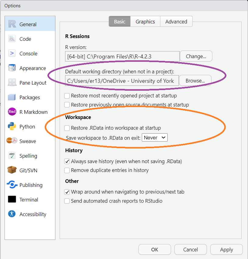
First, we will set our default working directory. Under ‘Default working directory (when not in a project²):’ click Browse and navigate to a through your file system to a folder where you want to work. You may want to create a folder specifically for studying this book.

Second, we will change the Workspace options. Turn off ‘Restore .RData into workspace at startup’ and change ‘Save workspace to .RData on exit’ to ‘Never’. These options mean R will start up clean each time.

7.1 Recap of RStudio anatomy

This figure (see Figure 7.2³) summarises shows what each of the four RStudio panes and what they are used for to summarise much of what we have covered so far.

Figure 7.2: A screenshot of RStudio’s four panes annotated with what each pane is for. You can zoom into this at the Direct link

7.2 Data types and structures in R

In this section, we are going to introduce you to some of R’s data types and structures. We won’t be covering all of them now, just those you are going to use often in this part of the book. These are numerics (numbers), characters, ‘logicals’, vectors and dataframes. We can do a lot with just these. We will also cover using functions.

We are going to consider

• types of value also known as data types

• functions

• data structures

7.2.1 Data types

This refers to the type of value that something is. They might be numerics or characters or ‘logical’ (either true of false). We assign a number, like the value of 23 to a variable called x like this:

x <- 23
x
## [1] 23

We do not need to use quotes for numbers but we do need to use them for characters and can assign the word banana to the variable a like this:

a <- "banana"
a
## [1] "banana"

Quotes are needed because otherwise R wouldn’t know whether you were referring to a value or a existing object called banana. This is also why you can’t have variable name like 14 - R would not be able to tell the difference between the number 14 and an object named 14 since numbers and objects don’t need quotes.

Anything composed of non-numeric characters, including single characters, need to have quotes around it. You can even force a number to be a character by putting quotes around it:

b <- "23"
b
## [1] "23"

Notice that things inside quotes appear in a different colour (the colour will depend on the Editor theme you choose). This will help you identify when you have forgotten some closing quotes:

a <- "banana
x <- 23

Notice how the x <- 23 is in the same colour as the string “banana” because we forgot to close the quotes. RStudio makes it hard for you to forget closing quotes and parentheses because when you type an opening quote or parenthesis, it automatically adds its closing partner. When people are learning they are sometimes tempted to delete these so they can type what goes inside the quotes/parentheses and then manually add the closing partner. I strongly recommend you do not delete them. RStudio adds the closing character but it leaves your cursor in the right position to complete the contents.

Although the data type is ‘character’ we often use the term ‘string’ for collections - strings - of characters

We also have special values called ‘logicals’ which take a value of either TRUE or FALSE.

c <- TRUE
c
## [1] TRUE

Although TRUE is a word, R recognises it as special word. It appears in a different colour and no quotes are needed. This is the same for FALSE.

c <- FALSE
c
## [1] FALSE

As you type FALSE, the colour changes as it recognises the special word FALSE. Try to pay attention to the editor theme’s colouring - it is trying to help you!

7.2.2 Functions

The aim of this section is to help you understand the logic of using a function. Functions have a name and then a set of parentheses. The function name minimally explains what the function does. Inside the parentheses are ‘arguments’ - the pieces of information you give to the function. When coding, we often talk about passing arguments to functions and calling functions. A simple function call looks like this:

function_name(argument)

A function can take zero to many arguments. Where you give several arguments, they are separated by commas:

function_name(argument1, argument2, argument3, ...)

The first function you are going to use is str() which gives the structure of an object:

str(x)
##  num 23

It’s telling me that x is a number and contains 23.

Your turn! Use str() on b:

str(b)
##  chr "23"

str() is a function I use a lot to check what sort of R object I have.

We must give str() at least one argument, the object we want the structure of, but additional arguments are also possible. Later we will discover how to find out and use a function’s arguments.

So far we our objects have consisted of a single thing but usually we have several bits of data that we want to collect together into a data structure.

7.2.3 Data structures: vectors

Imagine we have the ages of six people. Since all the numbers are ages, we would want to keep them together. The minimal data structure is called a vector. We can create a vector, which collects together several numbers using a function, c(). This is one of only a few functions in R with a single-letter name. Because it has a single letter, sometimes people get confused about it but we can tell it is a function because it has a set of parentheses.

To create a vector called ages of several numbers we use

ages <- c(23, 42, 7, 9, 54, 12)

Type ages and run if you want to print the contents to the console:

ages
## [1] 23 42  7  9 54 12

Using str() on ages

str(ages)
##  num [1:6] 23 42 7 9 54 12

tells us we have numbers with the indices of 1 to 6.

We can also create a vector of strings. Suppose we have names to go with the ages.

names <- c("Rowan", "Aang", "Zain", "Charlie", "Jules", "Efe")

RStudio has a super useful feature for putting items in quotes, brackets or parentheses if you initially forget them: If you select something and type the opening element, that thing will be surrounded rather than over written. For example, if you had written:

names <- Rowan, Aang, Zain, Charlie, Jules, Efe

Select one of the names and then type an opening quote - you should see the name is then surrounded by quotes rather than overwritten. You can repeat this process for all the names (note that double clicking on the name will select it). Selecting the whole list and typing an opening parenthesis will put the whole list in parentheses. This is a feature you get to love so much and use so often that other programs will annoy you when you overwrite something you meant to quote!

So we can also have vectors of logical values. For example, we might have a vector that indicates that Rowan, Aang and Charlie like chocolate, but Zain, Jules and Efe do not:

chocolate <- c(TRUE, TRUE, FALSE, TRUE, FALSE, FALSE)

Remember, because TRUE and FALSE are special words we do not need quote them.

7.2.4 Indexing vectors

You might be wondering how to get a single element out of a vector if typing the vector’s name prints the entire vector. This is by ‘indexing’. An index is a number from 1⁴ to the length of a vector which gives the position in the vector and is denoted by square brackets. For example, to pull out the second element of ages:

ages[2]
## [1] 42

Your turn! Print the last element of names:

names[6]
## [1] "Efe"

We an extract more than one element by giving more than one index. If the indices are adjacent like 3rd, 4th and 5th, we have use the colon:

names[3:5]
## [1] "Zain"    "Charlie" "Jules"

If the indices are not adjacent, like 2 and 6 with need to combine them with c():

names[c(2, 6)]
## [1] "Aang" "Efe"

We can also use a logical vector to extract elements. Suppose you want to extract the names and ages of the people who like chocolate:

names[chocolate]
## [1] "Rowan"   "Aang"    "Charlie"
ages[chocolate]
## [1] 23 42  9

At each of the indices in chocolate that contain TRUE, the name and age are returned.

7.2.5 Changing the defaults for a function

The functions we have used so far, c() and str() have worked without us having to change default behaviour. For example, if we want to calculate the mean age of our people we can use the mean() function in default form:

mean(ages)
## [1] 24.5

Imagine Charlie would like their age removed from the dataset or that we never knew their age. We would not want a vector containing just five elements because the ages would not match the people in the same position in the vector. Instead, we would have a missing value at that position. Missing values are NA (not applicable) in R and NA is another special word, like TRUE and FALSE, that doesn’t need quotes. We can set Charlie’s age to NA using indexing:

ages[names == "Charlie"] <- NA
ages
## [1] 23 42  7 NA 54 12

The == means “is equal to” and the result of names == "Charlie" is a vector of logicals: FALSE FALSE FALSE TRUE FALSE FALSE. This means ages[names == "Charlie"] references the age in ages at the index of Charlie in names

If we now try to calculate the mean age:

mean(ages)
## [1] NA

We get an NA! What we really want is an average of the ages we do have. The mean() function has an argument that allows you to cope with that situation called na.rm. By default, na.rm is set to FALSE but we can set it to TRUE using

mean(ages, na.rm = TRUE)
## [1] 27.6

7.2.6 Data structures: dataframes

We have three vectors, names, ages and chocolate which are all part of the same dataset. By far the most common way of organising data in R is within a “dataframe”. A dataframe, has rows and columns: each column represents a variable and each row represents a case. To make a dataframe using our three vectors we use:

people <- data.frame(names, ages, chocolate)

You will see people listed in the Global environment under Data. To open a spreadsheet-like view of the dataframe click its name in the Global Environment Figure 7.3

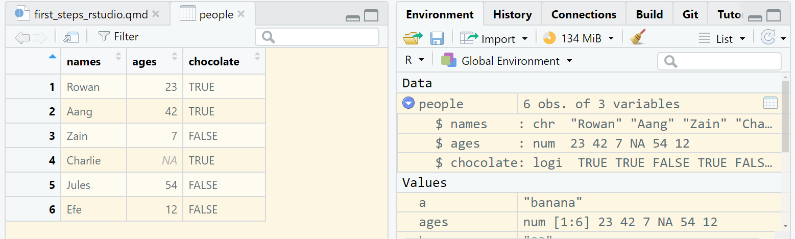
Figure 7.3: A screenshot of RStudio showing the people dataframe over the script on the left and the Environment pane on the right To open a spreadsheet-like view of the dataframe click its name in the Global Environment.

7.3 Install your first R package

We will be using the tidyverse (Wickham et al. 2019) package in this book.

Install tidyverse like this:

install.packages("tidyverse")

Installing a package means downloading it from the internet and placing its code on your computer. You only need to do this once – or each time you update your version of R. To use the package once it has been installed you need to load it with:

library(tidyverse)

Loading a package means telling R you want to use functions from that package in an R session. You need to load packages each time you start a new R session.

7.4 Summary

1. R can be used like a calculator. Commands are typed at the console prompt (>), and output appears below with line indices. Good practice includes using spaces around operators for readability.

2. Variables are created using <- (e.g., x <- 3). This is called assignment. These values can be reused in calculations, and errors (like using an undefined variable) are common and part of the learning process. Use the Environment tab and command history to track objects and troubleshoot.

3. Rather than typing directly into the console, use .R scripts to write and execute code. Scripts help keep a record of correct commands and allow comments (using #) to explain code.

4. Change some of the default RStudio settings: decide a default working directory and adjust workspace options to start clean each time (e.g., do not restore .RData on startup or save workspace on exit).

5. R uses basic data types like numeric, character (strings), and logical (TRUE/FALSE). Vectors are collections of values, created with c(). Indexing (e.g., ages[2]) retrieves elements by position or condition.

6. Functions take arguments in parentheses (e.g., mean(ages)). Some functions have default settings that can be changed (e.g., na.rm = TRUE to ignore missing values in mean()).

7. Data frame are rectangular and the most common structure for datasets in R.

Wickham, Hadley, Mara Averick, Jennifer Bryan, Winston Chang, Lucy D’Agostino McGowan, Romain François, Garrett Grolemund, et al. 2019. “Welcome to the tidyverse.” Journal of Open Source Software 4 (43): 1686. https://doi.org/10.21105/joss.01686.

---

1. When we are using scripts, it is very easy to write code but forget to run it. Very often when you see this error it will because you have written the code to create an object but forgotten to execute it.

2. We will find out what an RStudio Project is very soon. You will want to use a project for most of your work - they make everything a little easier.

3. You can zoom into this at the Direct link

4. We start counting from 1 in R. Most programming languages count from zero.