21 Pseudomonas putida grown in two soil types at two temperatures
You are reading a live document. This page is a dumping ground for one or more ideas. Sections maybe missing, or in bullet form and code may not be explained.
21.1 Scenario
Pseudomonas putida, is a hydrocarbon-degrading bacterium used for cleaning up oil-contaminated soil. P.putida was growth on either hexadecane contaminated or control soil at two temperatures: 4 degrees or 25 degrees. The was is to determine the effect of temperature and soil type on the number of bacteria in the soil.
Each group in a large class did one replicate and added their data to a Google sheet: https://docs.google.com/spreadsheets/d/1k2Gq4tKGEI0v_tdfgI-1d-Lk4YaWAC50sHffOmnqESU/edit?gid=886771226#gid=886771226
file <- "https://docs.google.com/spreadsheets/d/1k2Gq4tKGEI0v_tdfgI-1d-Lk4YaWAC50sHffOmnqESU/edit?gid=886771226#gid=886771226"class_data <- read_sheet(file) |> janitor::clean_names()You will be asked to authenticate in your browser. This message will appear in the console and the browser should open
Waiting for authentication in browser...
Press Esc/Ctrl + C to abort
You can Allow “Tidyverse API Packages wants to access your Google Account”.
You might also be asked
Is it OK to cache OAuth access credentials in the folderChoose the option for yes
The httpuv package enables a nicer Google auth experience, in many cases, but it
isn't installed.
Would you like to install it now?
Choose the option for yes.
The data should then read in.
read_sheet() from googlesheets4
Next time you run read_sheet() from googlesheets4 you will not have to authenticate in your browser if you chose “yes” for Is it OK to cache OAuth access credentials in the folder.
Instead you will see:
The googlesheets4 package is requesting access to your Google account.
Enter '1' to start a new auth process or select a pre-authorized account.
1: Send me to the browser for a new auth process.
2: your.email@whereever.ac.uk
You can chose 2
We don’t need the timestamp or group name columns and these can be dropped using the select() command
The data are in wide format - there is sample in column. We want to convert to long format so that each row contains a single count and the other columns give the soil and the temperature treatment. We can use pivot_longer() for this.
Drooping the columns (-) and pivoting the data can be done in one pipeline:
class_data <- class_data |>
  select(-timestamp, -group_name) |>
  pivot_longer(cols = everything(),
               names_to = "treatment",
values_to = "counts_cpg") ggplot(class_data,
aes(x = soil, y = counts_cpg, fill = temp)) +
geom_boxplot() 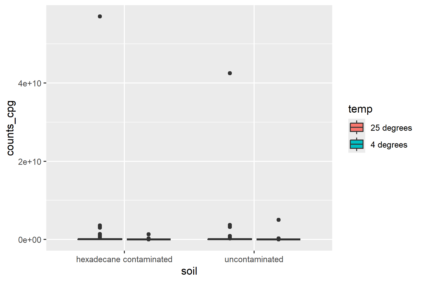
The data are not normally distributed - there are a few very large values. Logging the data will aid visualisation:
ggplot(class_data,
       aes(x = soil, y = log10(counts_cpg), fill = temp)) +
geom_boxplot() 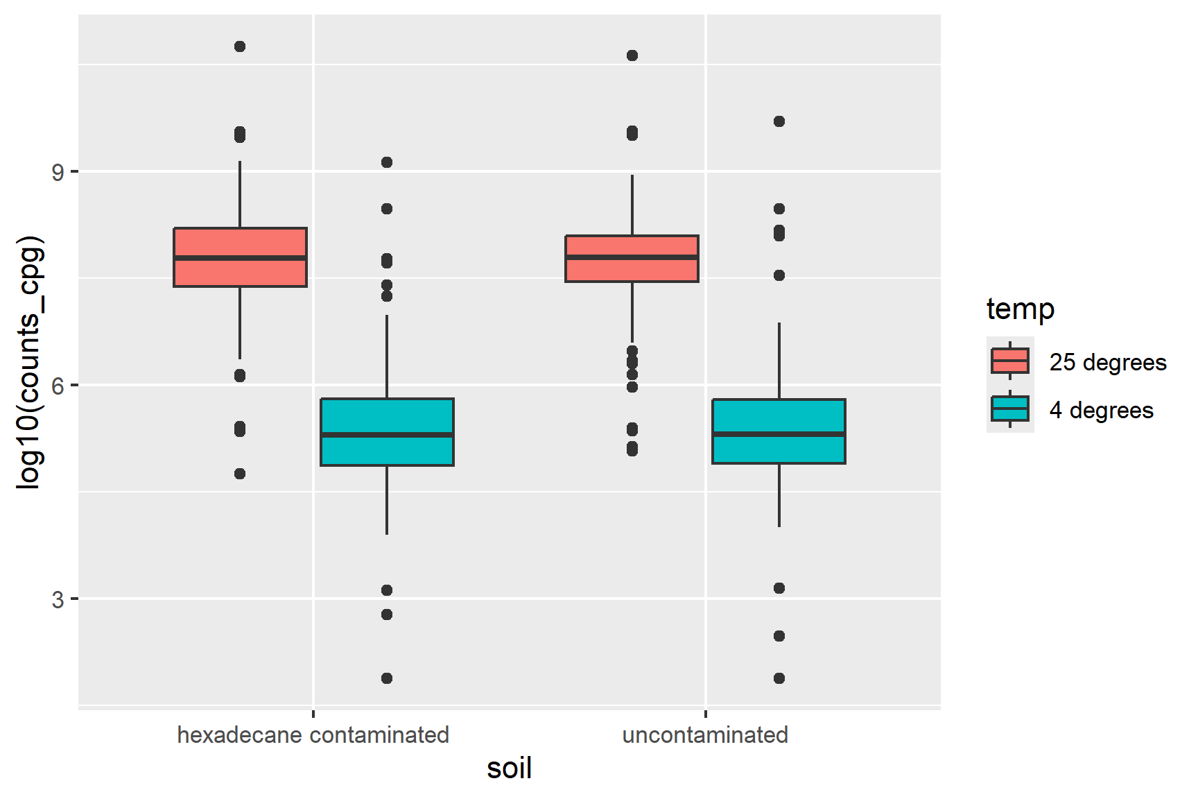
That’s better but the warning: Removed 11 rows containing non-finite outside the scale range indicates that there are some zeros. We can add 1 to the counts before logging to avoid this. This is a common practice. It is useful because log(1) = 0 which simplifies interpretation and is better than removing them. Many of the values are very large - the next smallest number is 75 - and adding 1 to large values before logging will have very little impact.
ggplot(class_data,
       aes(x = soil, y = log10(counts_cpg + 1), fill = temp)) +
geom_boxplot() 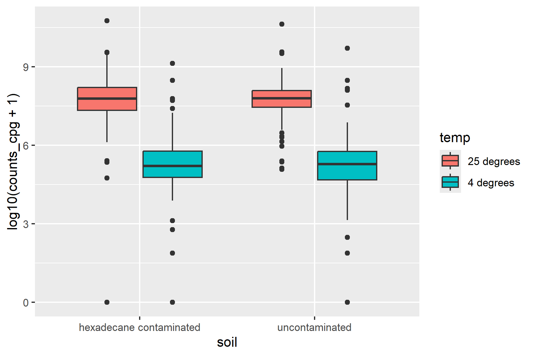
Temperature seems to matter but there is little difference between the two soils. The difference between the two temperatures is about the same in both soils suggesting no interaction.
Add a new column to the data frame with the logged values that we can use in the model.
Summarise the data to get the means and se for each group.
two-way anova
mod <- lm(data = class_data,
log_counts ~ soil * temp)summary(mod)
##
## Call:
## lm(formula = log_counts ~ soil * temp, data = class_data)
##
## Residuals:
## Min 1Q Median 3Q Max
## -7.631 -0.275 0.184 0.618 4.655
##
## Coefficients:
## Estimate Std. Error t value
## (Intercept) 7.59990 0.15895 47.81
## soiluncontaminated 0.03141 0.22479 0.14
## temp4 degrees -2.58646 0.22479 -11.51
## soiluncontaminated:temp4 degrees 0.00356 0.31791 0.01
## Pr(>|t|)
## (Intercept) <0.0000000000000002 ***
## soiluncontaminated 0.89
## temp4 degrees <0.0000000000000002 ***
## soiluncontaminated:temp4 degrees 0.99
## ---
## Signif. codes: 0 '***' 0.001 '**' 0.01 '*' 0.05 '.' 0.1 ' ' 1
##
## Residual standard error: 1.54 on 372 degrees of freedom
## Multiple R-squared: 0.416, Adjusted R-squared: 0.411
## F-statistic: 88.2 on 3 and 372 DF, p-value: <0.0000000000000002anova(mod)
## Analysis of Variance Table
##
## Response: log_counts
## Df Sum Sq Mean Sq F value Pr(>F)
## soil 1 0 0 0.04 0.83
## temp 1 628 628 264.41 <0.0000000000000002 ***
## soil:temp 1 0 0 0.00 0.99
## Residuals 372 884 2
## ---
## Signif. codes: 0 '***' 0.001 '**' 0.01 '*' 0.05 '.' 0.1 ' ' 1There is a strong and significant effect of temperature, no effect of soil and no interaction between temperature and soil. The effect of temperature is independent of soil.
examine the assumptions
ggplot(mapping = aes(x = mod$residuals)) +
geom_histogram(bins = 30) 
Too may values in the middle, too few in the shoulders for a normal distribution.
shapiro.test(mod$residuals)
##
##  Shapiro-Wilk normality test
##
## data:  mod$residuals
## W = 0.82, p-value <0.0000000000000002
Significantly different from a normal distribution.
plot(mod, which = 1)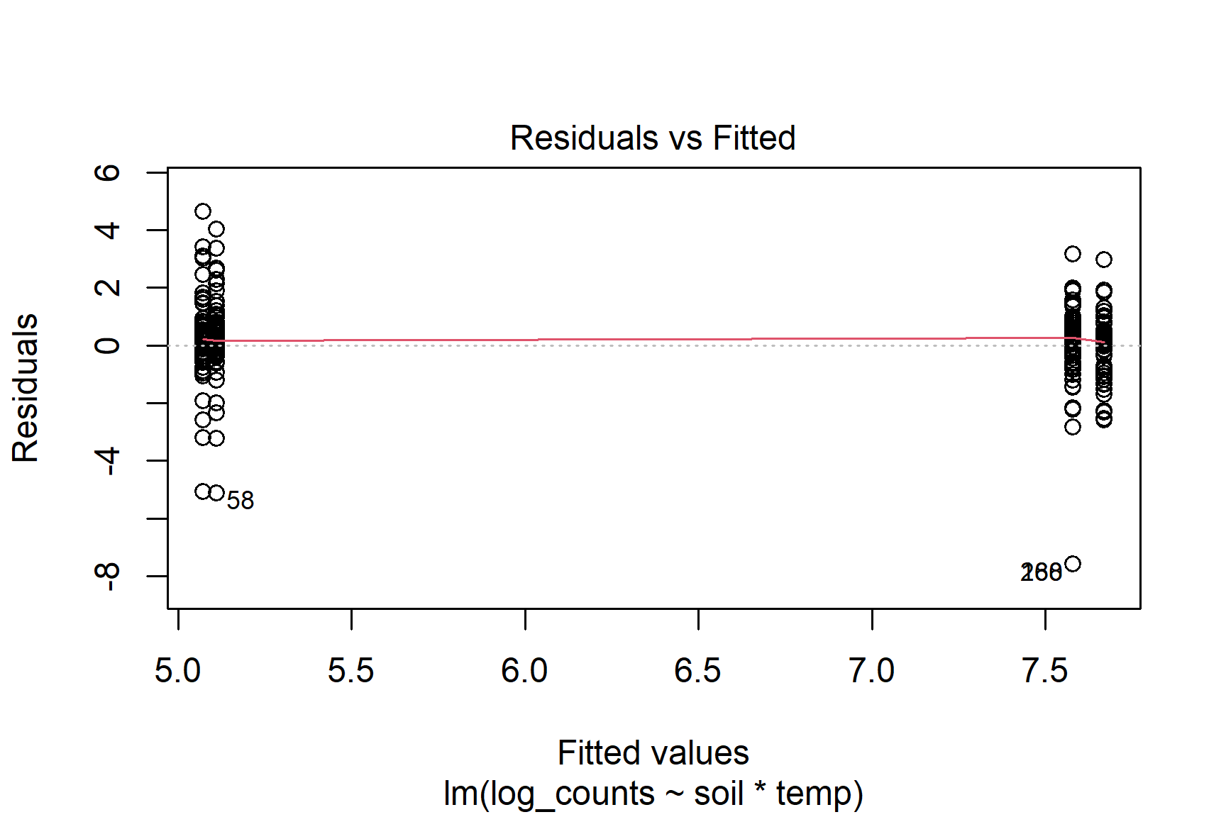
Variances are similar in each group
Not normal but reasonably symmetrical and variances are similar in each group. In addition, the effect is very clear - not at all borderline - so this case I will continue with the two-way anova.
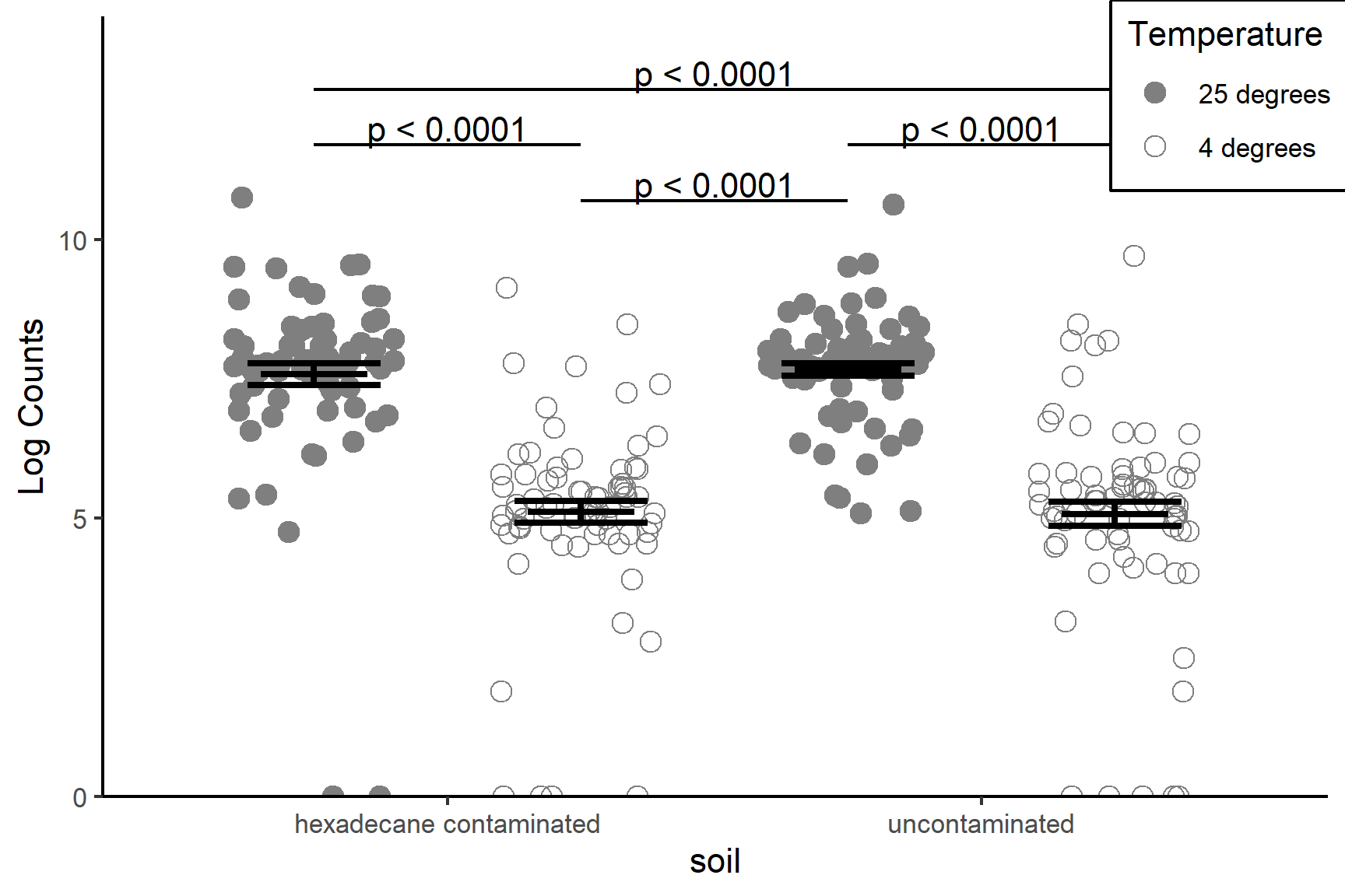
Post-hoc tests. Expecting differences between temps regardless of soil type.
emmeans(mod, ~ soil * temp) |> pairs()
##  contrast
##  hexadecane contaminated 25 degrees - uncontaminated 25 degrees
##  hexadecane contaminated 25 degrees - hexadecane contaminated 4 degrees
##  hexadecane contaminated 25 degrees - uncontaminated 4 degrees
##  uncontaminated 25 degrees - hexadecane contaminated 4 degrees
##  uncontaminated 25 degrees - uncontaminated 4 degrees
##  hexadecane contaminated 4 degrees - uncontaminated 4 degrees
##  estimate    SE  df t.ratio p.value
##   -0.0314 0.225 372  -0.140  0.9990
##    2.5865 0.225 372  11.506  <.0001
##    2.5515 0.225 372  11.350  <.0001
##    2.6179 0.225 372  11.646  <.0001
##    2.5829 0.225 372  11.490  <.0001
##   -0.0350 0.225 372  -0.156  0.9987
##
## P value adjustment: tukey method for comparing a family of 4 estimates
ggplot() +
  geom_point(data = class_data,
             aes(x = soil, y = log_counts, shape = temp),
             position = position_jitterdodge(dodge.width = 1,
                                             jitter.width = 0.3,
                                             jitter.height = 0),
             size = 3,
             colour = "gray50") +
  geom_errorbar(data = class_data_summary,
                aes(x = soil, ymin = mean - se,
                    ymax = mean + se, group = temp),
                width = 0.5,
                linewidth = 1,
                position = position_dodge(width = 1)) +
  geom_errorbar(data = class_data_summary,
                aes(x = soil, ymin = mean, ymax = mean, group = temp),
                width = 0.4,
                linewidth = 1,
                position = position_dodge(width = 1) ) +
  scale_x_discrete(name = "soil", expand = c(0, 0)) +
  scale_y_continuous(name = "Log Counts", expand = c(0, 0),                                                                                                              limits = c(0, 14)) +
  scale_shape_manual(values = c(19, 1),
                     name = "Temperature") +
  # hexadecane contaminated 25 degrees -
  # hexadecane contaminated 4 degrees <.0001
  annotate("segment",
           x = 0.75, xend = 1.25,
           y = 11.7, yend = 11.7,
           colour = "black") +
  annotate("text", x = 1, y = 12,
           label = "p < 0.0001") +
  # uncontaminated 25 degrees -
  # uncontaminated 4 degrees <.0001
  annotate("segment",
           x = 1.75, xend = 2.25,
           y = 11.7, yend = 11.7,
           colour = "black") +
  annotate("text", x = 2, y = 12,
           label = "p < 0.0001") +
  # hexadecane contaminated 25 degrees -
  # uncontaminated 4 degrees <.0001
  annotate("segment",
           x = 0.75, xend = 2.25,
           y = 12.7, yend = 12.7,
           colour = "black") +
  annotate("text", x = 1.5, y = 13,
           label = "p < 0.0001") +
  # uncontaminated 25 degrees -
  # hexadecane contaminated 4 degrees <.0001
  annotate("segment",
           x = 1.25, xend = 1.75,
           y = 10.7, yend = 10.7,
           colour = "black") +
  annotate("text",
           x = 1.5, y = 11,
           label = "p < 0.0001") +
  theme_classic() +
  theme(legend.position = "inside",
        legend.position.inside = c(0.92, 0.9),
        legend.background = element_rect(colour = "black"))