11 The logic of hypothesis testing
Complete
You are reading a live document. This page is compete but suggestions for improvements are welcome. Follow the link to ‘Make a suggestion’ to suggest improvements.
11.1 What is Hypothesis testing?
Hypothesis testing is a statistical method that helps us draw conclusions about a population based on a sample. Since we usually can’t measure every individual in a population, we instead take a smaller sample and make inferences about the population.
For example, suppose we want to know if knocking out gene X in cultured cells changes the expression level of protein Y compared to the established wild‑type mean. Measuring expression in every cell would be impractical, so we take a sample. However, even if the knockout has no real effect, our sample’s average expression might differ from the wild‑type reference just by chance. Hypothesis testing helps us determine whether this difference is real or just random variation.
11.2 Samples and populations
Before we dive deeper into hypothesis testing, let’s clarify two key terms:
- A population is the entire group we are interested in studying (e.g., all possible knockout cells cultures).
- A sample is a smaller group selected from the population (e.g., a 10 samples of cells cultured for the study).
We use samples because studying an entire population is often impractical. This means making sure our sample accurately represents the population.
11.3 Logic of hypothesis testing
The logic behind hypothesis testing follows these general steps:
- Formulating a “Null Hypothesis” denoted \(H_0\). The null hypothesis is what we expect to happen if nothing interesting is happening. It states that there is no difference between groups or no relationship between variables. In our case, \(H_0\) is that the mean expression of protein Y in the knockout cells equals that of the wild‑type. In contrast, the “Alternative Hypothesis” (\(H_1\)) states that there is a significant difference between the knockout mean and wild-type reference
- Designing an experiment and collecting data to test the null hypothesis.
- Finding the probability (the p-value) of getting our experimental data, or data as extreme or more extreme, if \(H_0\) is true.
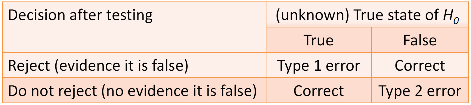
- Deciding whether to reject or not reject the \(H_0\) based on that probability:
- If \(p ≤ 0.05\) we reject \(H_0\)
- If \(p > 0.05\) do not reject \(H_0\)
If the null hypothesis is rejected it means we have evidence that \(H_0\) is untrue and support for \(H_1\). If the null hypothesis is not rejected, it means there is insufficient evidence to support the alternative hypothesis. It is important to recognise that not rejecting \(H_0\) does not mean it is definitely true – it just indicates that \(H_0\) cannot be discounted.
Whatever our test result, there is a real state to \(H_0\), that is, \(H_0\) is either true or it is not true. The statistical test has us decide whether to reject or not reject \(H_0\) based on the p-value. This means we can make mistakes when testing a hypothesis. These are called Type I and Type II errors.
11.3.1 Type I and type II errors
Type I and type II errors describe the cases when we make the wrong decision about the null hypothesis. These errors are inherent in the approach rather than mistakes you can prevent.
- A type I error occurs when we reject a null hypothesis that is true. This can be thought of as a false positive. It is a real error in that we conclude there is a real difference or effect when there is not. Since we use a probability of 0.05 to reject the null hypothesis, we will make a type I error 5% of the time.
- A type II error occurs when we do not reject a null hypothesis that is false – a false negative. It is not a real error in the sense that we only conclude we do not have enough evidence to reject the null hypothesis. We do not claim the null hypothesis is true.
- If we reject a null hypothesis that is false we have not made an error.
- If we do not reject a null hypothesis that is true we have not made an error.
We can decrease our chance of making a type I error by reducing the the p-value required to reject the null hypothesis. However, this will increase our chance of making a type II error. We can decrease our chance of making a type II error by collecting enough data. The amount of data needed will depend on the the size of the effect relative to the random variation in the data.
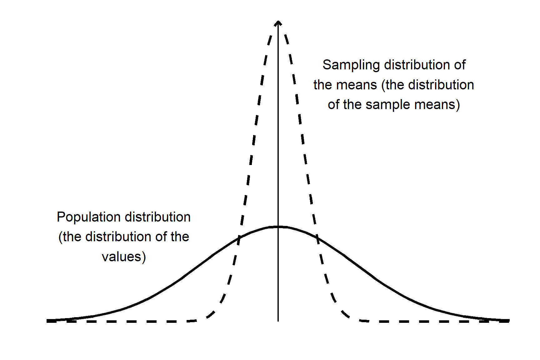
11.4 Sampling distribution of the mean
The sampling distribution of the mean is a fundamental concept in hypothesis testing and constructing confidence intervals. Parametric tests such as regression, two-sample tests and ANOVA (all applied with lm()) are all based on the sampling distribution of the mean. It is a theoretical distribution that describes the distribution of the sample means if an infinite number of samples were taken.
The key characteristics of the sampling distribution of the mean are:
The mean of the sampling distribution of the mean is equal to the population mean
The standard deviation of the sampling distribution of the mean is known the standard error of the mean and is always smaller than the standard deviation of the values. There is a fixed relationship between the standard deviation of a sample or population and the standard error of the mean: \(s.e. = \frac{s.d.}{\sqrt{n}}\)
As the sample size increases, the sampling distribution of the mean becomes narrower and and more peaked around the population mean. As the sample size decreases the sampling distribution of the mean becomes wider and closer to the population distribution.
💡 Why does this matter? It matters because when we calculate a p-value, what we really want to know is: “How likely is it to get a sample mean like this (or one as extreme or more extreme) if \(H_0\) is true. That is, it is the distribution of the sample means that we are interested in, not the distribution of the values.
11.4.1 Example
Let’s work through this logic using our example.
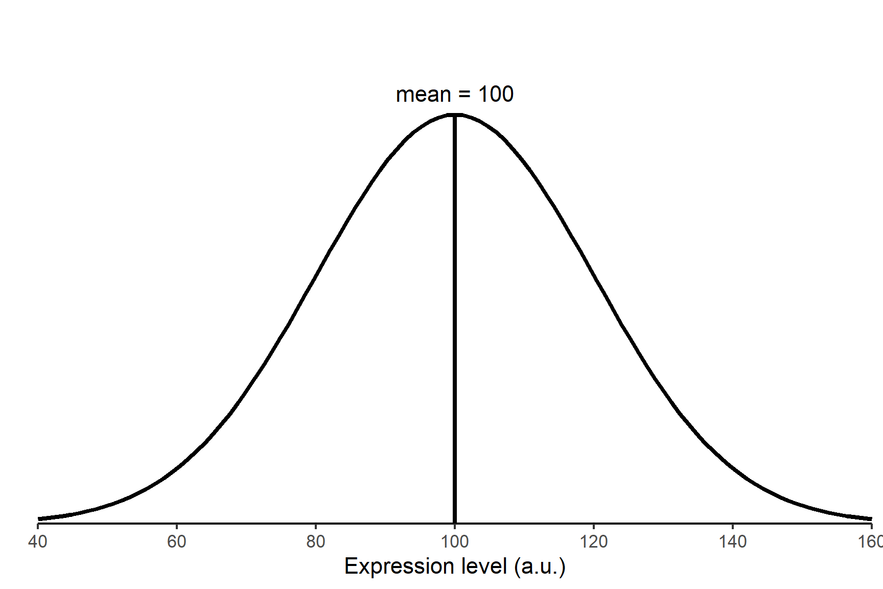
Question: The wild‑type mean expression of protein Y is 100 a.u. with a standard deviation of 20 a.u. If we knock out gene X, does the mean expression change?
- Set up the null hypothesis. The null hypothesis is what we expect to happen if nothing interesting is happening. In this case, that there is no effect of knocking out gene X, i.e., the mean of a sample of knockout cell cultures is equal to wild‑type mean of 100 a.u. (Figure 11.3). This is written as \(H_0: \bar{x}\) = 100. The alternative hypothesis is that the sample mean is not equal to wild‑type mean of 100 a.u. This is written as \(H_1: \bar{x} \neq\)
Design an experiment that generates data to test the null hypothesis. We take a sample of \(n\) = 10 knockout cell cultures and determine the mean protein Y expression. Suppose we calculate \(\bar{x}\) = 92. This is lower than the wild-type population mean but might we get such a sample even if the null hypothesis is true?
Determine the probability (the p-value) of getting our experimental data , or data as extreme or more extreme, if \(H_0\) is true. This would be a mean of 92 or less
OR a mean of 108 or more (Figure 11.4). This is because 108 a.u. is just as far away from the expected value as 92 a.u.
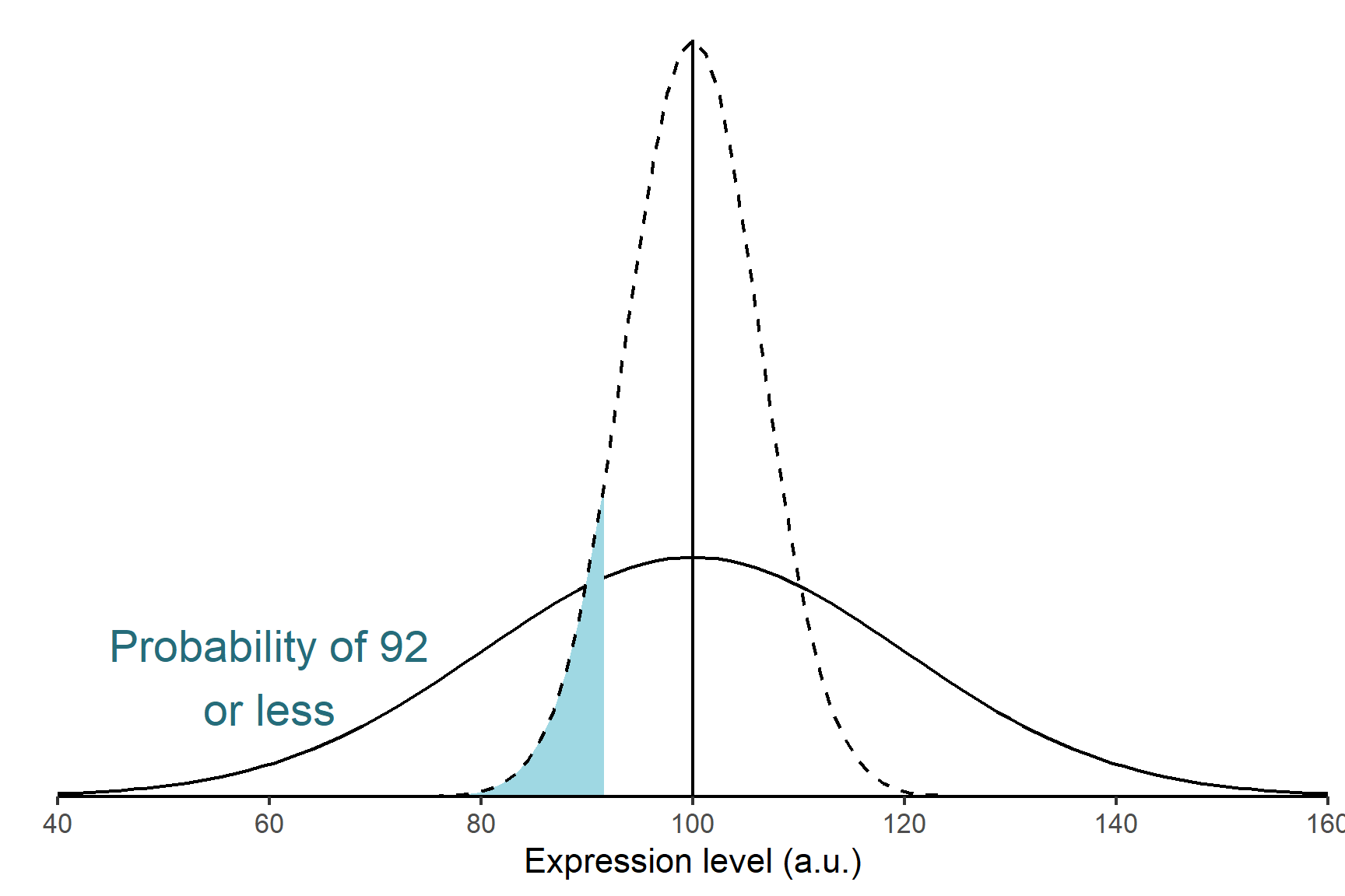
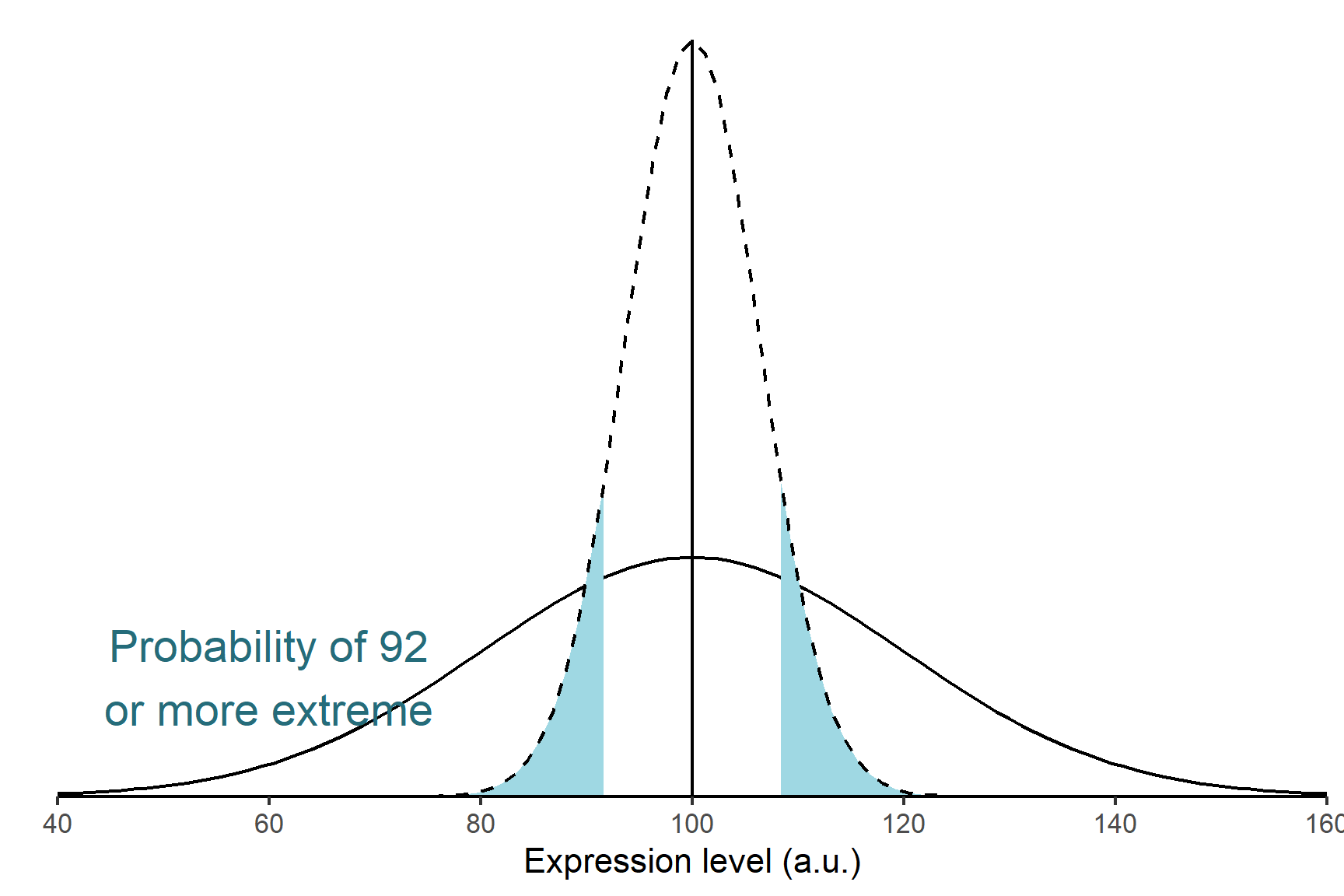
- Decide whether to reject or not reject the \(H_0\) based on that probability. If the shaded area is less than 0.05 we reject the null hypothesis and conclude there is a difference between the mean of the knockout cell cultures and the wild‑type cultures. If the shaded area is more than 0.05 we do not reject the null hypothesis.
11.5 Summary
Hypothesis testing is a statistical method that helps us draw conclusions about a population based on a sample.
A population is the full set of entities possible; a sample is a random subset of the population.
The logic of hypothesis testing involves formulating a null hypothesis, designing an experiment, calculating the probability of obtaining the observed data if the null hypothesis is true, and deciding whether to reject or not reject the null hypothesis based on that probability.
That probability is determined by the sampling distribution of the mean. This is a theoretical distribution that describes the distribution of sample means if an infinite number of samples were taken. It has a mean equal to the population mean and a standard deviation known as the standard error of the mean.
A type I error occurs when we reject a null hypothesis that is true, while a type II error occurs when we do not reject a null hypothesis that is false.