20 Molecular weight from SDS-PAGE
Draft
You are reading a live document. This page is a draft but is mainly complete should be readable.
20.1 Overview
Sodium Dodecyl Sulfate-Polyacrylamide Gel Electrophoresis (SDS-PAGE) is a method to separate proteins by size.
Proteins are denatured and coated with SDS (a detergent), giving them a uniform negative charge. They migrate through a polyacrylamide gel when an electric current is applied. The lower the molecular weight of the protein, the faster, and therefore further, it migrates through the gel. Gels are run with a “marker lane” containing proteins of known molecular weights. The positions of these marker proteins are used to create a “standard curve” that allows us to estimate the molecular weights of other proteins in the gel. The proteins are made visible by staining (e.g. with Coomassie Blue). SDS-PAGE can tell you the size of proteins in a sample, but not their identity. It can also be used to find the relative abundances of the proteins.
this section we will use a linear regression to estimate the molecular weights of proteins from an SDS-PAGE gel.
This is a different use for linear regression than the single linear regression we covered in Chapter 14. In that section we wanted to statistically test whether an x-variable explained the variation in a y-variable.
Here we already know there is a very tight linear relationship between the position of the marker proteins on the gel and their molecular weights. But here we are using the linear regression to find the equation of the line that describes this relationship so we can use it to estimate the molecular weights of other proteins in the gel.
We will explore all of these ideas with an example.
20.2 🎬 Your turn!
If you want to code along you will need to start a new RStudio Project (see Section 8.1.2), add a data-image folder and open a new script. You will also need to load the tidyverse package (Wickham et al. 2019).
20.3 Linear Regression for estimating molecular weights from gels
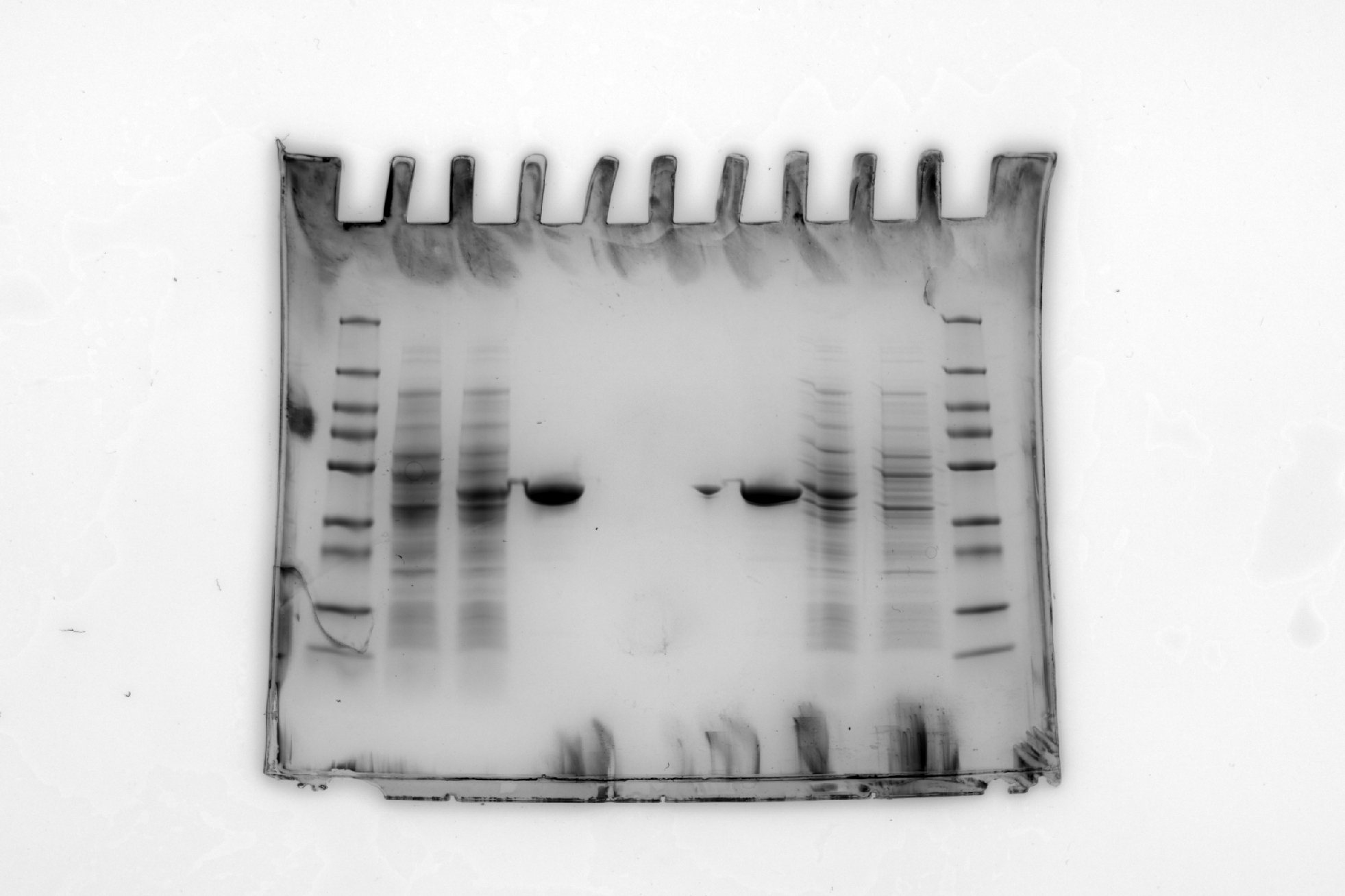
We will use this gel image (Figure 20.1) as an example: sds-page-gel.jpg. This gel has two sets of results (one each side) - since only 4 lanes were needed for each experiment, we put two experiments on one gel.
Lane 1 (and 10) is the protein ladder which are the proteins of known molecular weights.
Lane 2 (and 9) is Uninduced E. coli lysate
Lane 3 (and 8) is Induced E. coli lysate
Lane 4 (and 7) is ShPatB
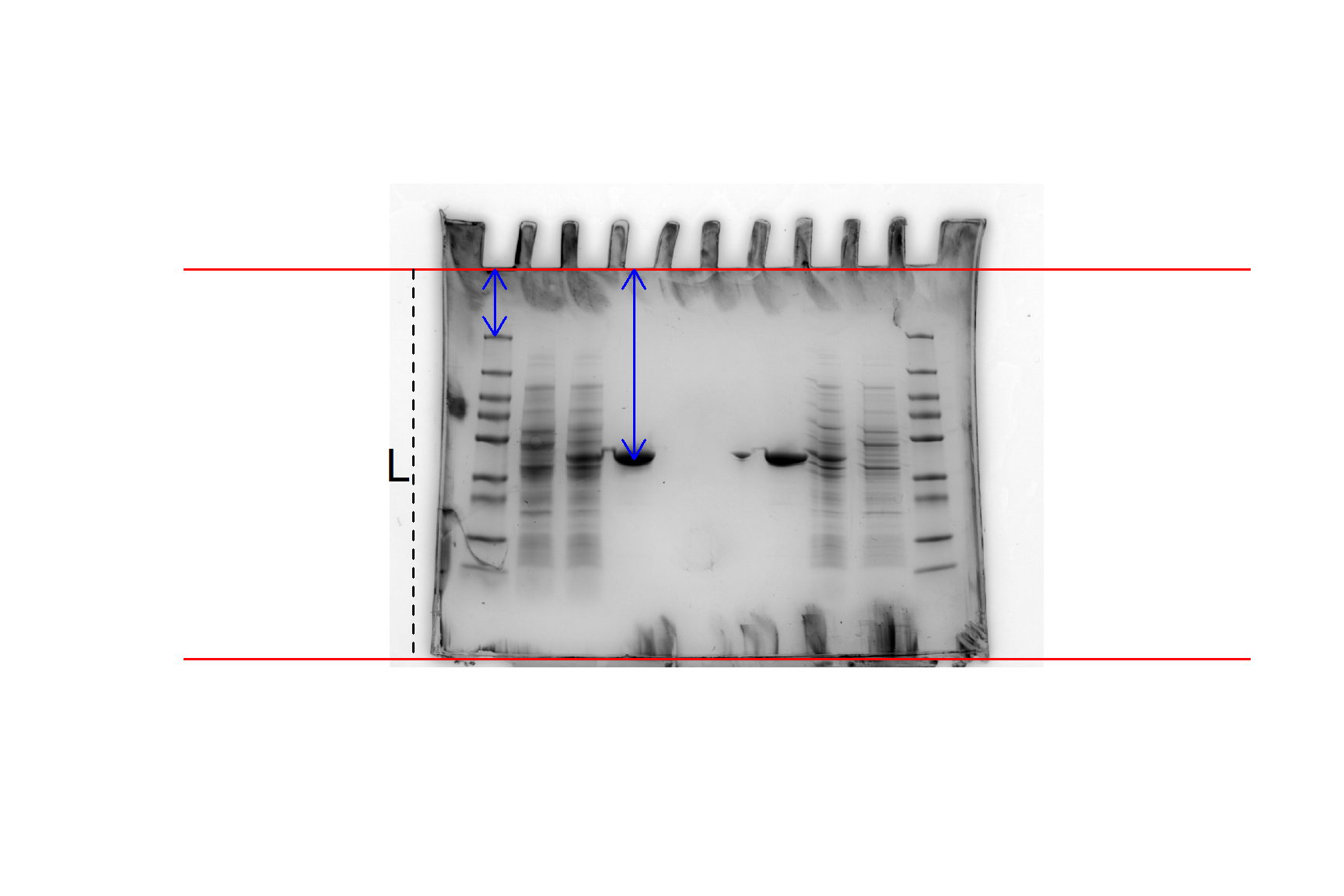
You don’t need worry about the details of the gel, only that our aim is to estimate the molecule weight of the ShPatB protein in lane 4 from its position on the gel and the standard curve created from the marker proteins in lane 1. Figure 20.1 illustrates the measurements needed from the gel image.
We will cover two options:
Where you have measured the length of the gel, the positions of ShPatB and the marker proteins on the gel manually - by opening the gel image in Powerpoint for example – and have a file containing the molecular weights and positions of the marker proteins. The measures can be in centimetres or pixels, it does not matter as long as they are all in the same units.
Where you have a file containing the molecular weights of the marker proteins and use R to measure the length of the gel, the positions of ShPatB and the marker proteins by importing the gel image. This method relies on the
locator()function which stores the coordinate positions when you click on a plot! Magic!
20.3.1 Option 1: Manual measurements
You have measured the positions of the marker proteins and added them to a file containing the molecular weights. Your file is: standard-mw-with-positions.csv. The molecular weights of the marker proteins are in kilodaltons (kDa) and the positions of the marker proteins are in pixels. The length of the gel is 810 pixels and ShPatB is at 394 pixels from the top of the gel.
Save standard-mw-with-positions.csv to data-raw/ and import it.
mw_positions <- read_csv("data-raw/standard-mw-with-positions.csv")Assign the position of ShPatB and the length of the gel to variables:
gel_length <- 810
pos_patB <- 394
We need to calculate \(R_f\) values for the marker proteins:
\[R_f = \frac{L - d}{L}\]
where \(L\) is the length of the gel and \(d\) is the distance to the band.
We also need to log the molecular weights of the marker proteins to make a linear relationship. We can add these two new variables to the data frame using the mutate().
Calculate \(R_f\) values for the marker proteins:
mw_positions <- mw_positions |>
  mutate(Rf = (gel_length - dist_to_band) / gel_length,
         log_kda = log(kda))
Plot the data with geom_point() and add a linear regression line with geom_smooth(method = "lm"):
ggplot(mw_positions, aes(x = Rf, y = log_kda)) +
  geom_point() +
  geom_smooth(method = "lm",
              se = FALSE) +
  theme_classic()
Fit a linear model so we have the equation of the line
mod <- lm(log_kda ~ Rf, data = mw_positions)Print the model:
mod
##
## Call:
## lm(formula = log_kda ~ Rf, data = mw_positions)
##
## Coefficients:
## (Intercept)           Rf
##        1.09         5.23
We only need to print the coefficients - we don’t care about the statistical tests here. You can tell from the plot that the relationship is very tight and linear. The equation of the line is: \(MW\)= 5.231 \(\times R_f\) + 1.091
You can substitute the values of the coefficients and the \(R_f\) of ShpatB to find the log molecular weight of ShPatB. Or you can use the predict() function to do this for you.
Calculate the \(R_f\) of ShPatB:
patB_Rf = (gel_length - pos_patB) / gel_lengthPredict the molecular weight ShPatB:
patB_kda <- predict(mod, newdata = data.frame(Rf = patB_Rf)) |>
  exp()
patB_kda
##     1
## 43.69
20.3.2 Option 2: Measurements in R
You have a file containing the molecular weights of the marker proteins standard-mw.txt and the image of the gel sds-page-gel.jpg. The molecular weights of the marker proteins are in kilodaltons (kDa)
Make a folder call data-image and save sds-page-gel.jpg to it. Save standard-mw.txt to data-raw.
Import the molecular weights of the marker proteins from standard-mw.txt
mw <- read_csv("data-raw/standard-mw.txt")Load the imager package
Import the gel image:
gel <- load.image("data-image/sds-page-gel.jpg")Base R’s generic plot() function can handle image files and plot axes default. These are in pixels and will help us mark the top and bottom of the gel.
Plot the gel image:
plot(gel)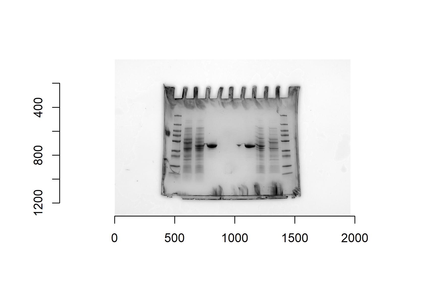
The imager package has a function that will crop the edges of the image. This is certainly not essential but can have two benefits:
- the image is smaller which means plotting is quicker – this is especially useful when your images are many pixels
- it makes it a little easier determine where the axes numbers are on the gel
Crop the image:
# crop
gel_cropped <- crop.borders(gel, nx = 300, ny = 150)
crop.borders() removes ny pixels from the top and the bottom and nx pixels from each side. You may wish to adjust the numbers.
Plot the cropped image:
plot(gel_cropped)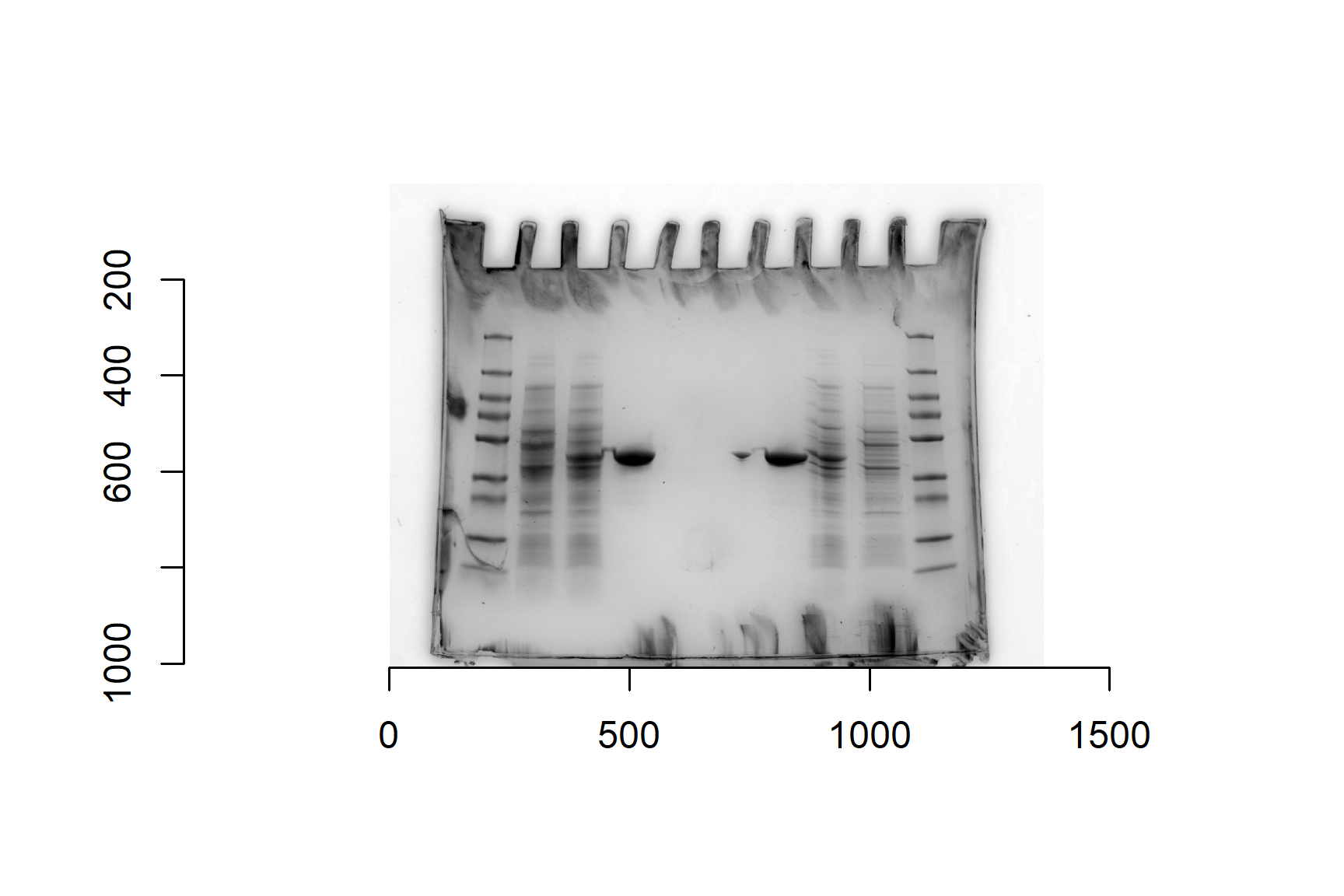
To make sure we measure distances from the same place we need to add lines to mark the top and the bottom of the gel. Notice that the y-axis is 0 at the top. I think the top is at about 180 and the bottom is about 990. We will assign these values to variables because they will be needed in calculations later. We will also need the gel length (bottom position - top position).
Assign values for the top and bottom of the gel to variables and calculate the length of the gel:
gel_top <- 180
gel_bottom <- 990
gel_length <- gel_bottom - gel_top
Plot the cropped gel with lines marking the top and bottom of the gel:
# plot gel
plot(gel_cropped)
# add a horizontal lines for the top and bottom of the gel
abline(h = gel_top, col = "red")
abline(h = gel_bottom, col = "red")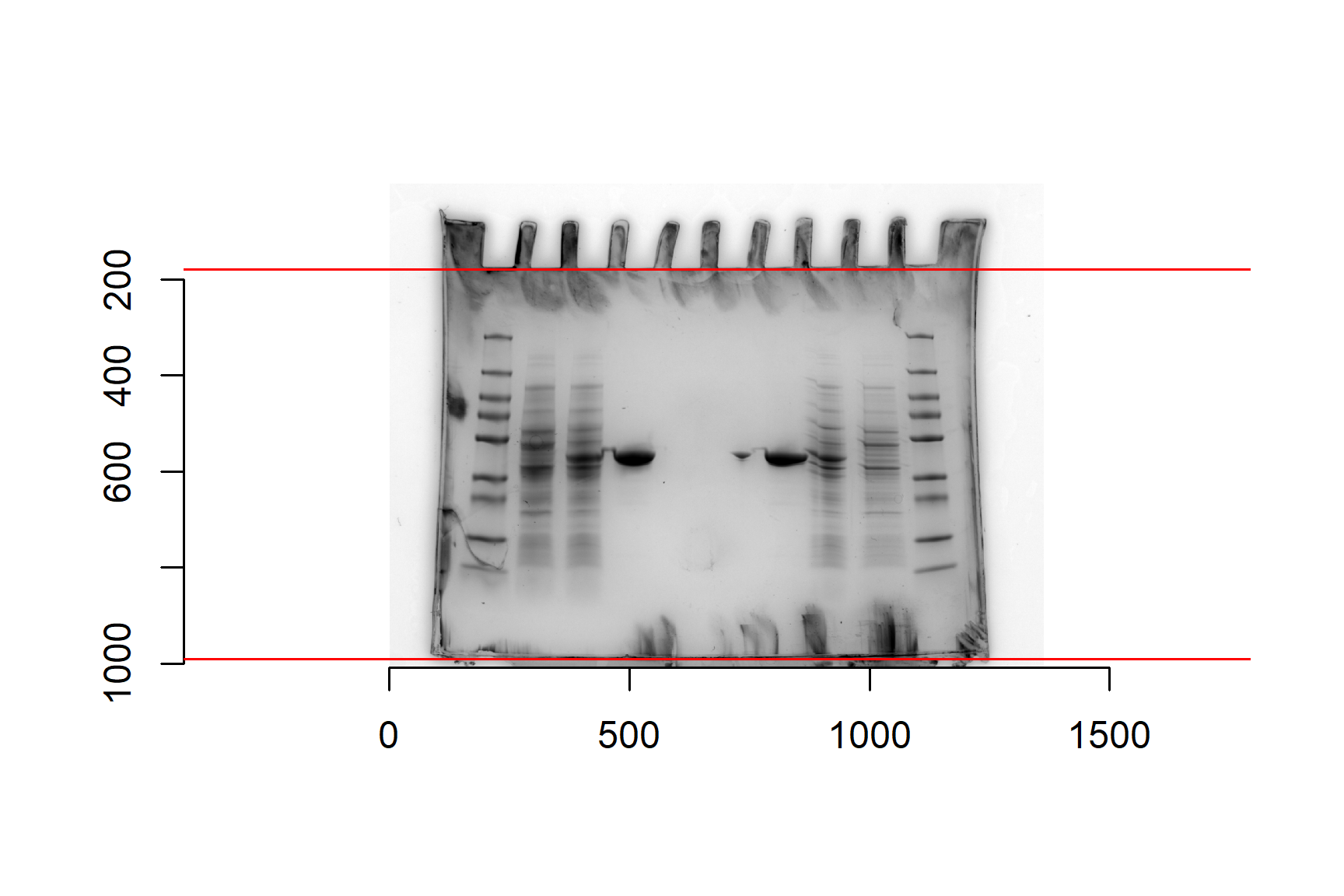
Make sure you run all these commands. The base plotting system works a little differently than ggplot. We do not use + but we have to make sure we have recently run the plot() command before the abline() (and other functions that modify plots) will work. You will get Error in int_abline(a = a, b = b, h = h, v = v, untf = untf, ...) : plot.new has not been called yet if you have not recently run the plot() command.
At this point you have check that you are happy with the numbers used for the top and bottom of the gel. Adjust and replot if needed.
I like to add a vertical line in the marker lane to help guide my later measures.
Add a vertical line in the marker lane. Again, make sure you run all of the plotting code:
# plot gel
plot(gel_cropped)
# add a horizontal lines for the top and bottom of the gel
abline(h = gel_top, col = "red")
abline(h = gel_bottom, col = "red")
# add a vertical line in the marker lane as a guide to help with locator
abline(v = 220, col = "red")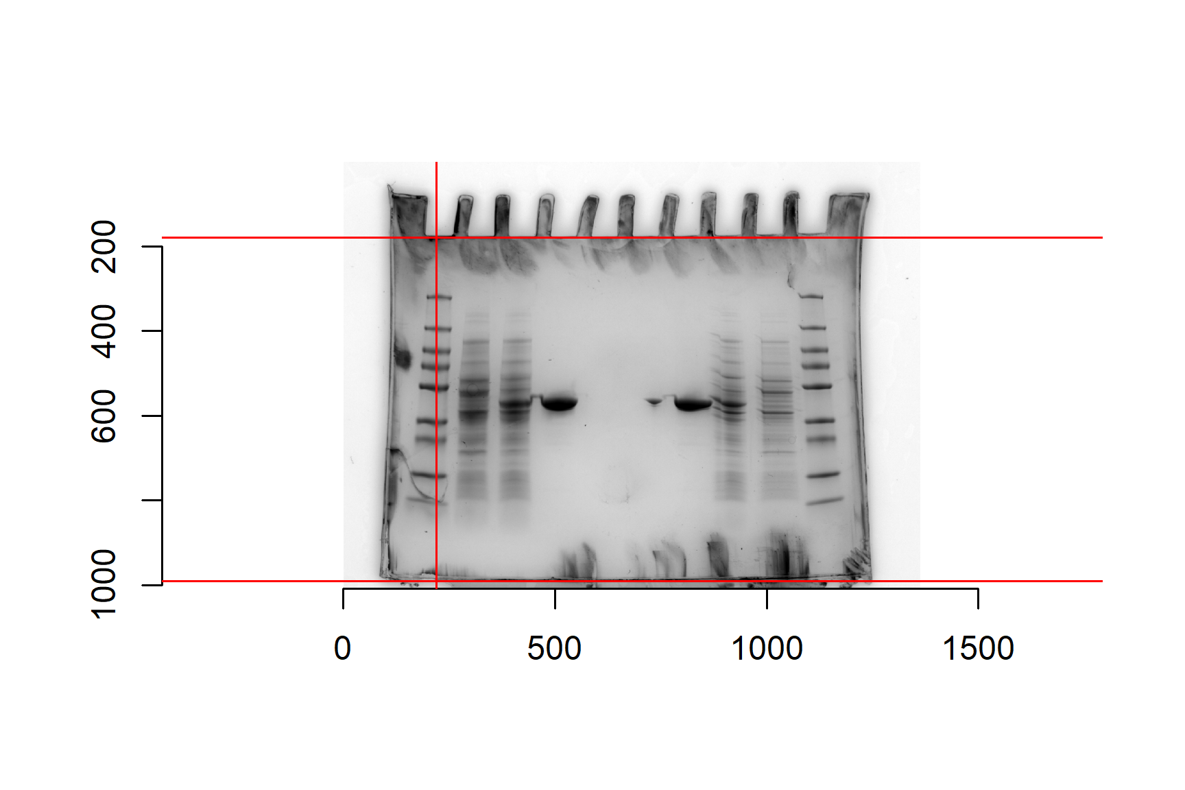
We are now ready to measure the band positions using the locator() function. We need to measure the position of shPatB and the all the marker proteins. We will start with shPatB:
Run the locator() command and click on the shPatB in lane 4:
dist_to_patB <- locator(n = 1)The (x,y) position of shPatB is now stored in an R object called pos_patB.
The distance between the shPatB band and the top of the gel will be the y value in dist_to_patB minus the distance to the top of the gel.
Calculate the distance from the top of the gel to shPatB:
pos_patB <- dist_to_patB$y - gel_topWe have 9 bands so pass the argument n = 9 to the function. This means you will need to click on the graph 9 times. Start at the top - the heaviest band - and work your way down. You only need to click once on each band. The R cursor will disappear until you have clicked 9 times. Don’t worry if you make a mistake, just click until the cursor is returned and run the locator command again to start afresh.
Run the locator() command and click on the 9 bands in order from top to bottom:
# Number of bands in your marker lane
# click from the top or gel to the bottom
# i.e., high MW to low
marker_positions <- locator(n = 9)
Magic! The (x,y) position of each band is now stored in an R object called marker_positions.
We need to
- combine the y positions with molecular weights in
mw - calculate the distance to each band by subtracting
gel_top - calculate \(R_f\) values for the marker proteins using \(R_f = \frac{L - d}{L}\) where \(L\) is the length of the gel and \(d\) is the distance to the band.
- log the molecular weights of the marker proteins to make a linear relationship.
We can put all these new columns in a dataframe called mw_positions frame using the mutate().
Create mw_positions from mw and the y positions in marker_positions:
mw_positions <- mw |>
  mutate(y = marker_positions$y,
         dist_to_band = y - gel_top,
         Rf = (gel_length - dist_to_band) / gel_length,
         log_kda = log(kda))
The process is now exactly the same as it was for Option 1.
Plot the data with geom_point() and add a linear regression line with geom_smooth(method = "lm"):
ggplot(mw_positions, aes(x = Rf, y = log_kda)) +
  geom_point() +
  geom_smooth(method = "lm",
              se = FALSE) +
  theme_classic()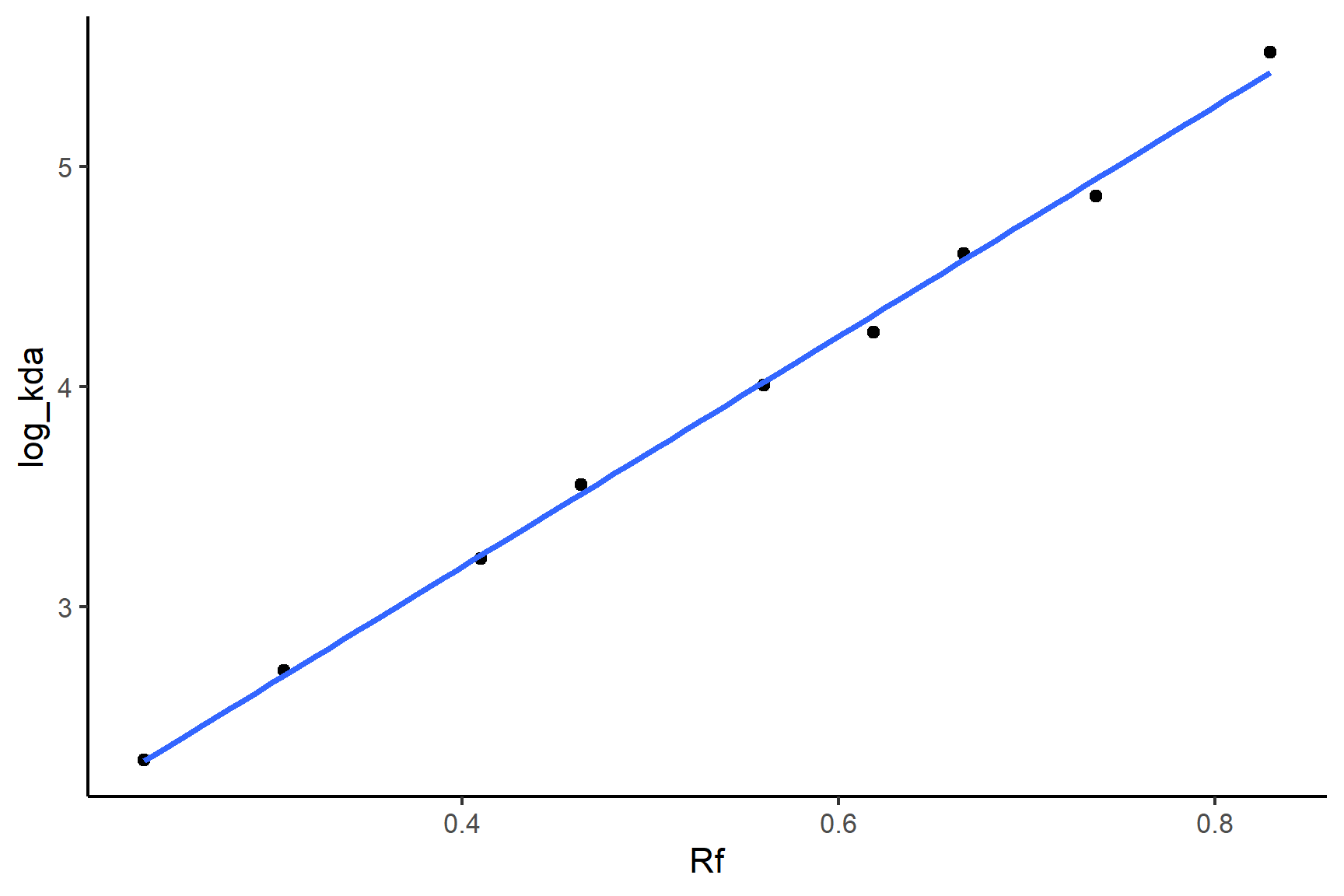
Fit a linear model so we have the equation of the line
mod <- lm(log_kda ~ Rf, data = mw_positions)Print the model:
mod
##
## Call:
## lm(formula = log_kda ~ Rf, data = mw_positions)
##
## Coefficients:
## (Intercept)           Rf
##        1.09         5.23
We only need to print the coefficients - we don’t care about the statistical tests here. You can tell from the plot that the relationship is very tight and linear. The equation of the line is: \(MW\)= 5.231 \(\times R_f\) + 1.091
You can substitute the values of the coefficients and the \(R_f\) of ShpatB to find the log molecular weight of ShPatB. Or you can use the predict() function to do this for you.
Calculate the \(R_f\) of ShPatB:
patB_Rf = (gel_length - pos_patB) / gel_lengthPredict the molecular weight ShPatB:
patB_kda <- predict(mod, newdata = data.frame(Rf = patB_Rf)) |>
  exp()
patB_kda
##     1
## 43.69
If you would like to practice Option 2 again, you could repeat the the steps using the set of results on the other side of the gel.
20.4 Summary
TO DO