plot(mod, which = 2)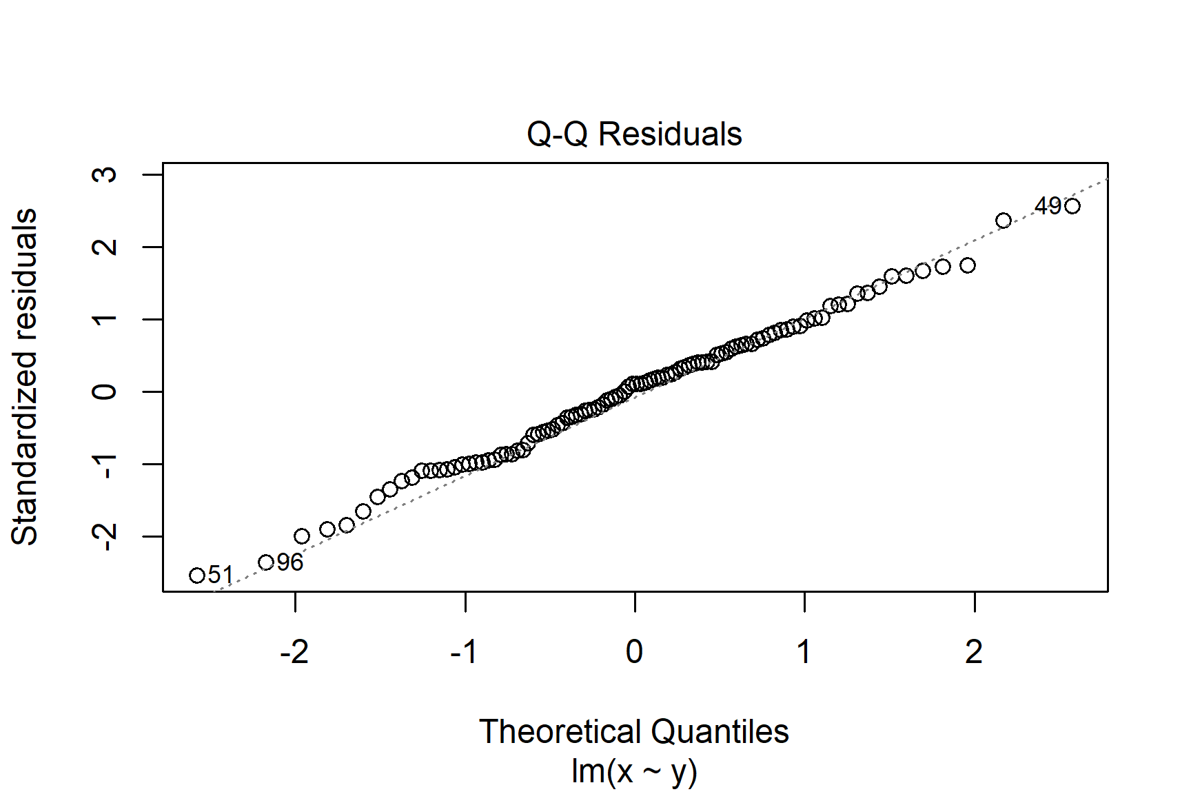
You are reading a work in progress. This page is compete but needs final proof reading.
This section discusses statistical models which are equations representing relationships between variables. Statistical models help us test hypotheses and make predictions. The process involves estimating model “parameters” from data and assessing “model fit”. Linear models include regression, t-tests, and ANOVA, known collectively as the General Linear Model. The assumptions of the general linear model are that the “residuals” are normally distribution and variance is homogeneous. If the assumptions are violated we can use non-parametric tests.
A statistical model is a mathematical equation that helps us understand the relationships between variables. We evaluate how well our data fit a particular model so we can infer something about how the values arose or make predictions about future values.
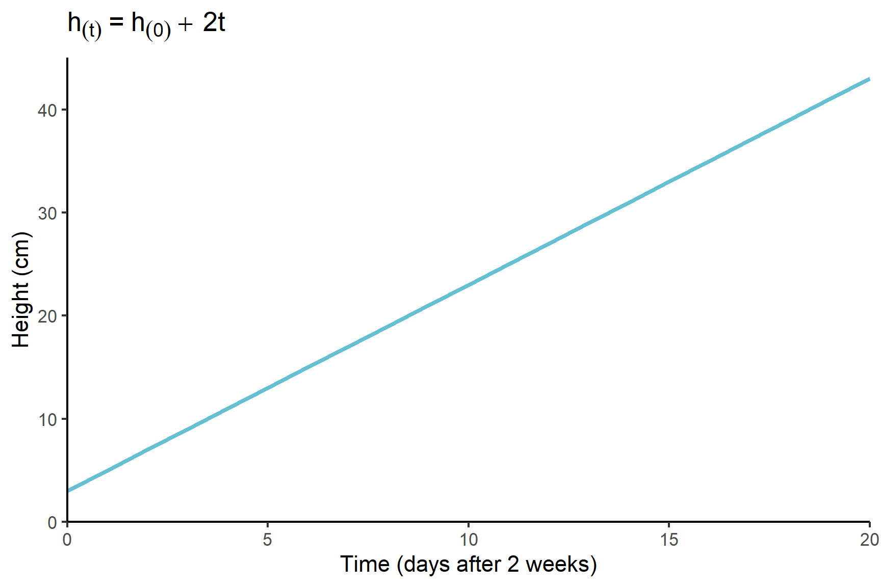
The equation states what has to be done to the explanatory values to get the response value. For example, a simple model of plant growth might be that a plant grows by 2 cm a day week after it is two weeks old. This model would be written as:
\[ h_{(t)} = h_{(0) }+ 2t \tag{11.1}\]
Where:
This model is a linear model because the relationship between the response variable, height, and the explanatory variable, time, is linear (See Figure 11.1 (a)). In a linear model, the gradient of the line is the same no matter what the value of \(t\). In this case, it is fixed at 2 cm per day.
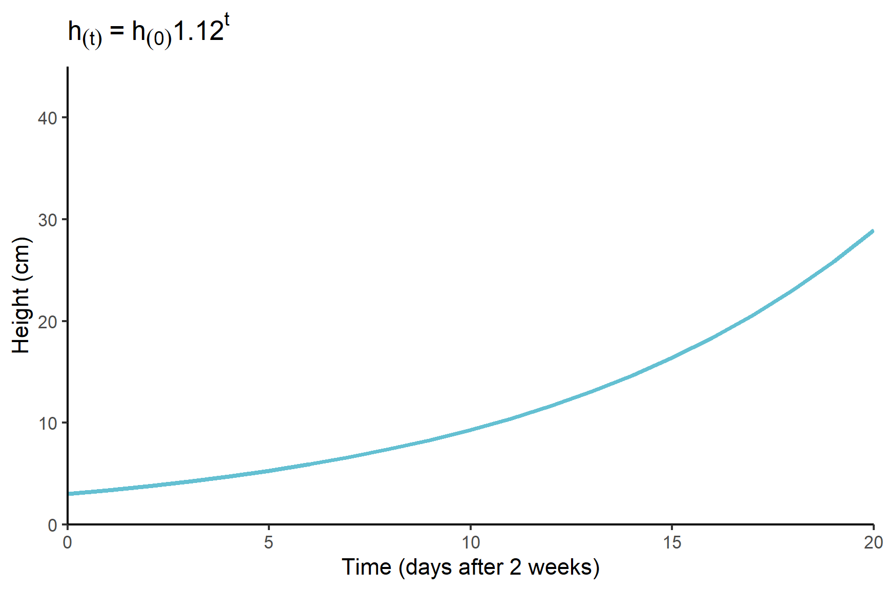
One alternative is a simple exponential model. In an exponential model, the height might increase by 12% each day and the gradient of the line would increase over time. This model is written as:
\[ h_{(t)} = h_{(0)}1.2^t \]
Where:
This model is not a straight line (See Figure 11.1 (b)). The gradient of the line increase as time goes on.
When we conduct statistical analysis, we are using a statistical model —a mathematical framework that describes the relationship between explanatory and response variables. Every model makes assumptions about this relationship, and we estimate the parameters of the model from the data. For example, in a simple linear model of plant growth, the key parameters are the intercept and the slope.
Statistical hypothesis testing is directly tied to these models. When we test a hypothesis, we are often assessing whether a particular model parameter is significantly different from zero. This is equivalent to testing whether an explanatory variable has an effect on the response variable.
In the context of hypothesis testing, the null hypothesis (\(H_0\)) typically states that a given parameter is equal to zero, meaning there is no effect or no relationship. The alternative hypothesis (\(H_1\)) suggests that the parameter is different from zero, indicating an effect.
To evaluate this, we calculate the probability of obtaining our estimated parameter value, or a more extreme value, if the true parameter were actually zero (i.e., if \(H_0\) were true). This probability is the p-value.
Because hypothesis tests depend on probability calculations, they also depend on certain assumptions about the data. A key assumption is that the estimated parameter follows a normal distribution, which allows us to use standard probability models to determine significance. This assumption is reasonable in many cases, but if it is violated, the p-values may be misleading.
For this reason, checking model assumptions is crucial. If the assumptions are not met, we might need to transform the data, choose a different model, or use non-parametric tests, which make fewer assumptions about data distribution. Non-parametric methods do not estimate parameters like an intercept and slope, which makes them useful when standard parametric assumptions are questionable.
Imagine we are studying a population of bacteria and want understand how nutrient availability influences its growth. We could grow the bacteria with different levels of nutrients and measure the diameter of bacterial colonies on agar plates in a controlled environment so that everything except the nutrient availability was identical. We could then plot the diameters against the nutrient levels.
We might expect the relationship between nutrient level and growth to be linear and add a line of best fit. See Figure 11.2.
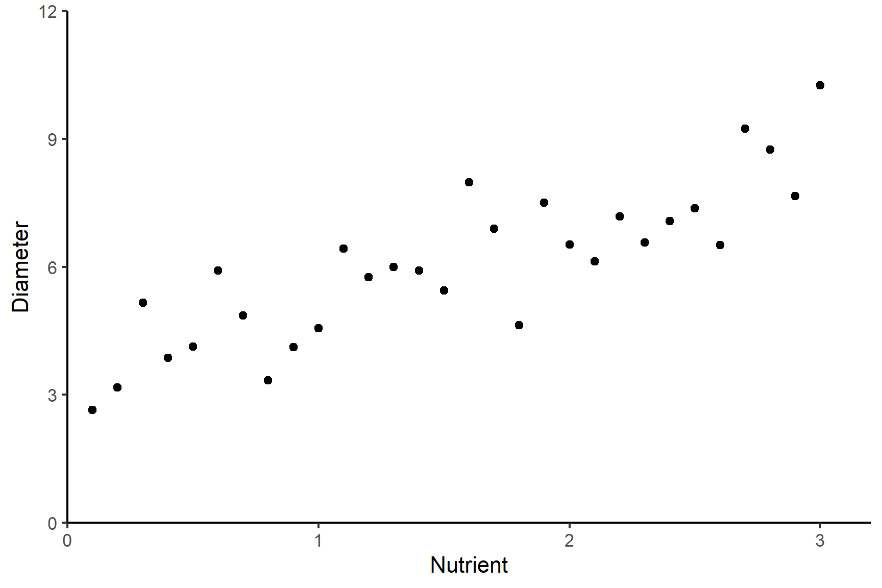
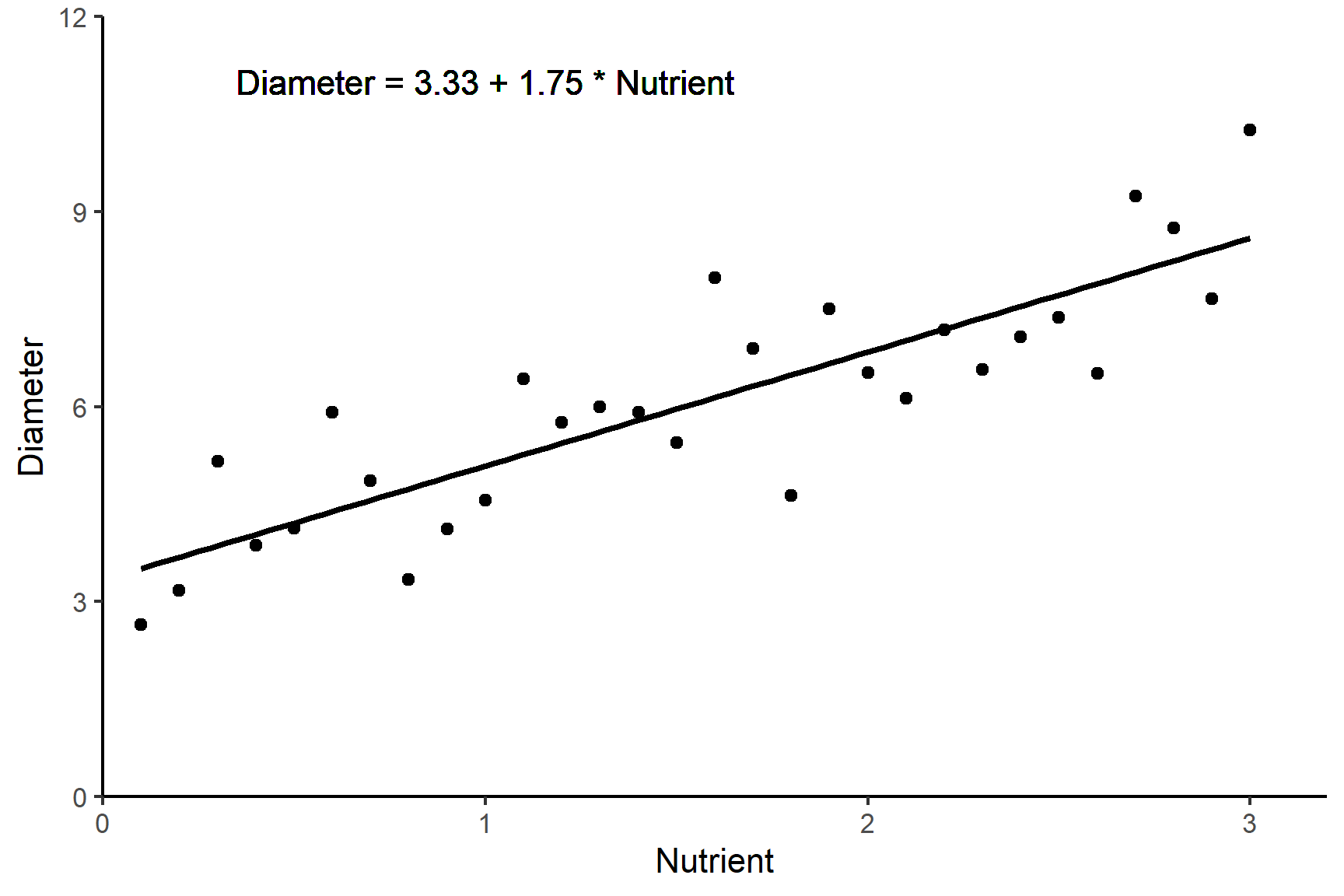
The equation of this line is a statistical model that allows us to make predictions about colony diameter from nutrient levels. A line - or linear model - has the form:
\[ y = \beta_{0} + \beta_{1}x \tag{11.2}\]
Where:
\(\beta_{0}\) and \(\beta_{1}\) are called the coefficients - or parameters - of the model.
In this case \[ Diameter = \beta_{0} + \beta_{1}Nutrient \tag{11.3}\]
Linear models are amongst the most commonly used statistics. Regression, t-tests and ANOVA are all linear models collectively known as the General Linear Model.
The process of estimating the parameters \(\beta_{0}\) and \(\beta_{1}\) from data is known as fitting a linear model. The line gives the predicted values of \(y\). The actual measured value of \(y\) will differ from the predicted value and this difference is called a residual or an error. The line is a best fit in the sense that \(\beta_{0}\) and \(\beta_{1}\) minimise the sum of the squared residuals, \(SSE\).
\[ SSE = \sum(y_{i}-\hat{y})^2 \tag{11.4}\]
Where:
Since \(\beta_{0}\) and \(\beta_{1}\) are those that minimise the \(SSE\), they are described as least squares estimates. You do not need to worry about this too much but it is a useful piece of statistical jargon to have heard of because it pops up often. The mean of a sample is also a least squares estimate - the sum of the squared differences between each value and the mean is smaller than the sum of the squared differences between each value and any other value.
The role played by \(SSE\) in estimating our parameters means that it is also used in determining how well our model fits our data. Our model can be considered useful if the difference between the actual measured value of \(y\) and the predicted value is small but \(SSE\) will also depend on the size of \(y\) and the sample size. This means we express \(SSE\) as a proportion of the total variation in \(y\). The total variation in \(y\) is denoted \(SST\):
\[ \frac{SSE}{SST} \tag{11.5}\]
\(\frac{SSE}{SST}\) is called the residual variation. It is the proportion of variance remaining after the model fitting. In contrast, the proportion of the total variance that is explained by the model is called R-squared, \(R^2\). It is:
\[ R^2=1-\frac{SSE}{SST} \tag{11.6}\]
If there were no explanatory variables, the value we would predict for the response variable is its mean. In other words, if you did not know the nutrient level for a randomly chosen bacterial colony the best guess you could make for its eventual diameter is the mean diameter. Thus, a good model should fit the response better than the mean - that is, a good model should fit the response better than a best guess. The output of lm() includes the \(R^2\). It represents the proportional improvement in the predictions from the regression model relative to the mean model. It ranges from zero, the model is no better than the mean, to 1, the predictions are perfect. See Figure 11.3

Since the distribution of the responses for a given \(x\) is assumed to be normal and the variances of those distributions are assumed to be homogeneous, both are also true of the residuals. It is our examination of the residuals which allows us to evaluate whether the assumptions are met.
See Figure 11.4 for a graphical representation of linear modelling terms introduced so far.

The assumptions of the general linear model are that the residuals are normally distributed and have homogeneity of variance. A residual is the difference between the predicted and observed value
If we have a continuous response and a categorical explanatory variable with two groups, we usually apply the general linear model with lm() and then check the assumptions, however, we can sometimes tell when a non-parametric test would be more appropriate before that:
To examine the assumptions after fitting the linear model, we plot the residuals and test them against the normal distribution
before: appropriate to the question, type of relationship. assumptions about the type of model
and after assumption calculations the probability calculations
implications of wrong choices: doesn’t anwser the question p value is inaccurate conclusions are wrong
We use the lm() function in R to analyse data with the general linear model. When you have one explanatory variable the command is:
lm(data = dataframe, response ~ explanatory)
The response ~ explanatory part is known as the model formula. These must be the names of two column in the dataframe.
When you have two explanatory variable we add the second explanatory variable to the formula using a + or a *. The command is:
lm(data = dataframe, response ~ explanatory1 + explanatory2)
or
lm(data = dataframe, response ~ explanatory1 * explanatory2)
A model with explanatory1 + explanatory2 considers the effects of the two variables independently. A model with explanatory1 * explanatory2 considers the effects of the two variables and any interaction between them. You will learn more about independent effects and interactions in Two-way ANOVA
We usually assign the output of an lm() command to an object and view it with summary(). The typical workflow would be:
 mod <- lm(data = dataframe, response ~ explanatory)

summary(mod)
There are two sorts of statistical tests in the output of summary(mod):
The F-test in the last line of the output indicates whether the relationship modelled between the response and the set of explanatory variables is statistically significant. i.e., whether it explains a significant amount of variation.
The assumptions relate to the type of relationship chosen and the hypothesis testing about the parameters. For a general linear model we assume the relationship between diameter and nutrients is linear and we examine this by plotting our data before running any tests.
The assumptions of the hypothesis testing in a general linear model are that residuals are normally distributed and have homogeneity of variance. A residual is the difference between the predicted and observed value. We usually check these assumptions after fitting the linear model by using the plot() function. This produces diagnostic plots to explore the distribution of the residuals. These cannot prove the assumptions are met but allow us to quickly determine if the assumptions are plausible, and if not, how the assumptions are violated and what data points contribute to the violation.
The two diagnostic plots which are most useful are the “Q-Q” plot (plot 2) and the “Residuals vs Fitted” plot (plot 1). These are given as values to the which argument of plot().
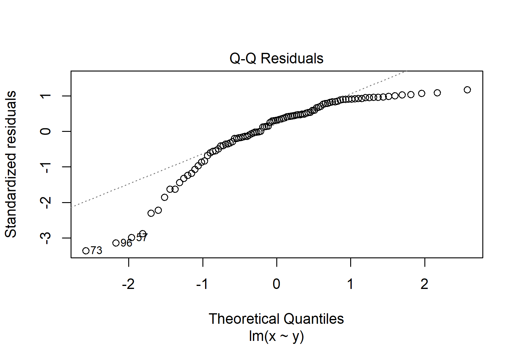
The Q-Q plot is a scatterplot of the residuals (standardised to a mean of zero and a standard deviation of 1) against what is expected if the residuals are normally distributed.
plot(mod, which = 2)
The points should fall roughly on the line if the residuals are normally distributed. In the example above, the residuals appear normally distributed.
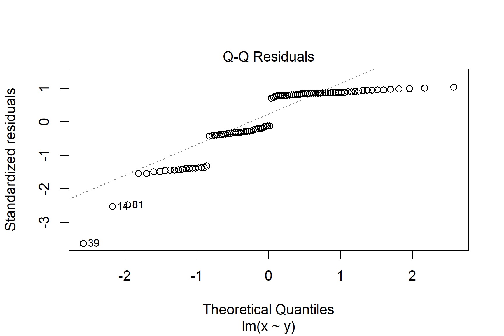
The following are two examples in which the residuals are not normally distributed.
If you see patterns like these you should find an alternative to a general linear model such as a non-parametric test or a generalised linear model. Sometimes, applying a transformation to the response variable will result in better meeting the assumptions.
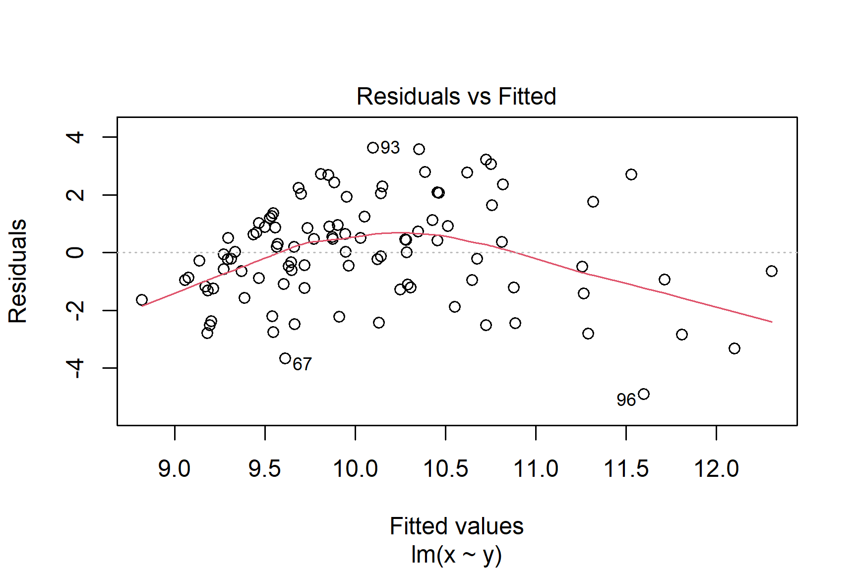
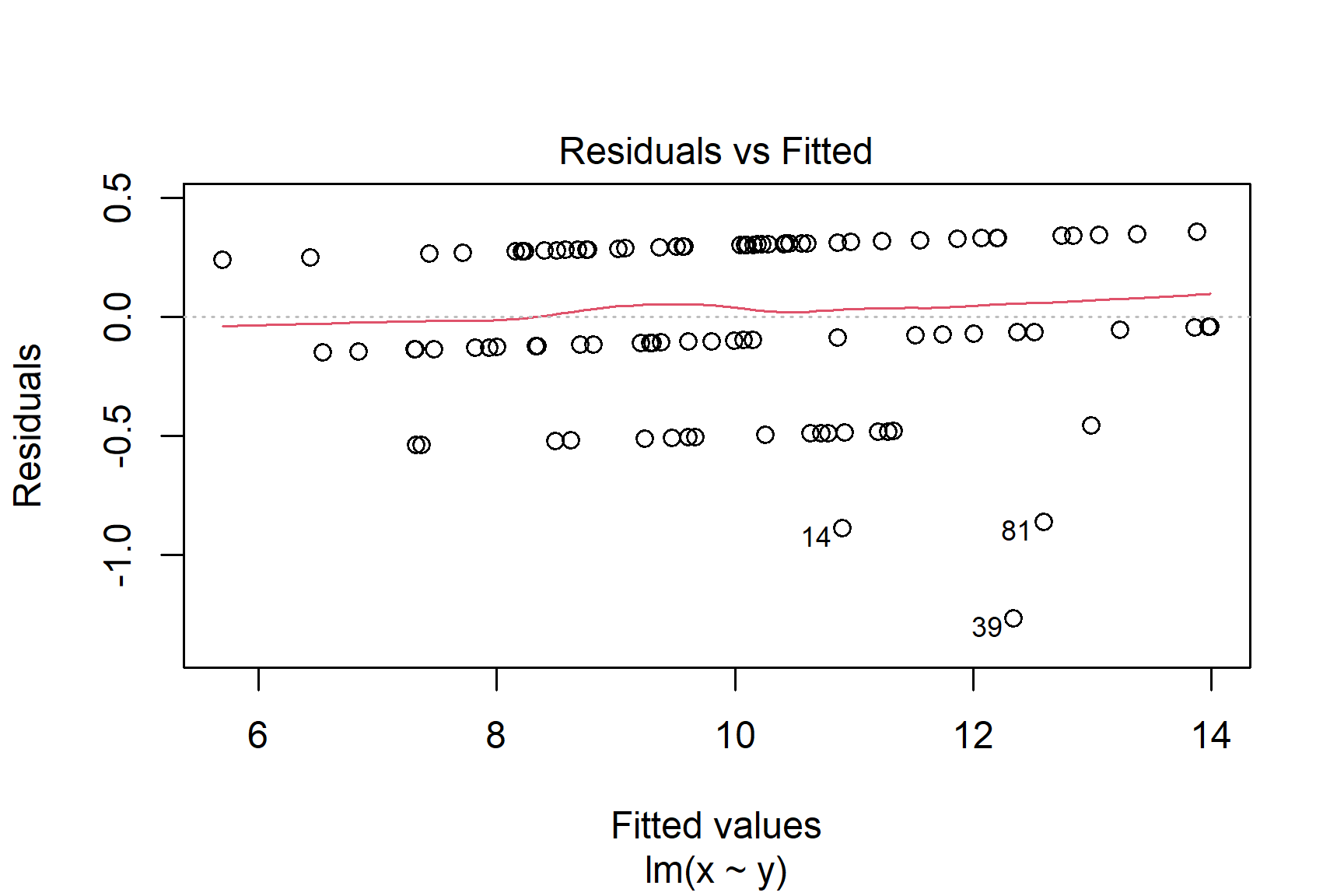
The Residuals vs Fitted plot shows if residuals have homogeneous variance or non-linear patterns. Non-linear relationships between explanatory variables and the response will usually show in this plot if the model does not capture the non-linear relationship. For the assumptions to be met, the residuals should be equally spread around a horizontal line as they are here:
plot(mod, which = 1)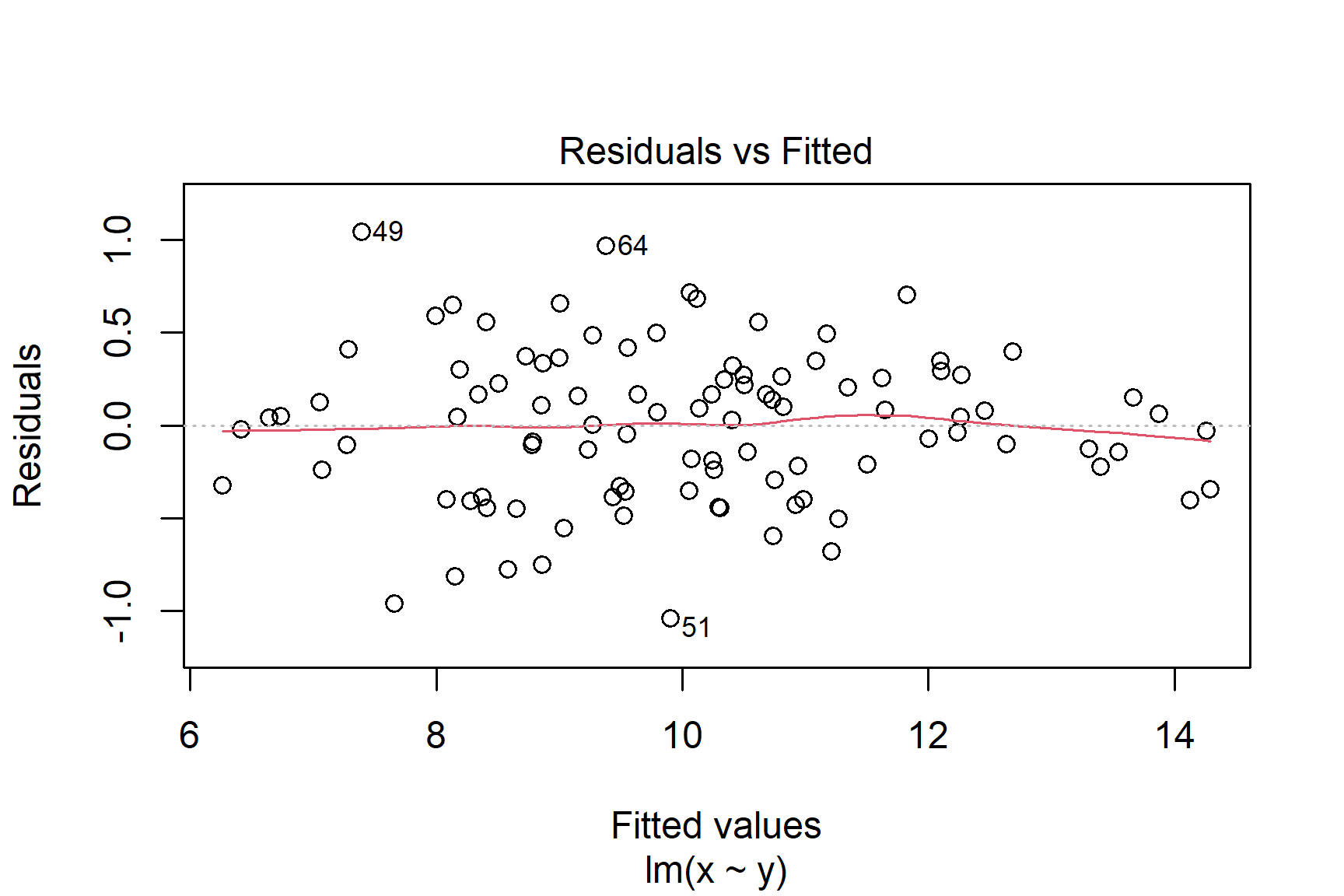
The following are two examples in which the residuals do not have homogeneous variance and display non-linear patterns.
When reporting the results of statistical tests we need to make sure we tell the reader everything they need to know and give the evidence it to support it. What they need to know is given in statements describing what difference or effect is significant and the evidence is from the test statistic and p-value from the test. You can think the statistical test values as being the evidence for the statements in your results sections, just as citations are the evidence for the statements in your introduction.
In reporting the result of a test we give:
the significance of effect
the direction of effect
the magnitude of effect
Figures should demonstrate the statement. Ideally they will include all the data and the ‘model’, i.e., the means and error bars or the fitted line. Figure legends should be concise but contain all the information needed to understand the figure. I like this blog on How to craft a figure legend for scientific papers
A statistical model is an equation that describes the relationship between a response variable and one or more explanatory variables.
A statistical model allows you to make predictions about the response variable based on the values of the explanatory variables.
Many statistical tests are types of “General Linear Model” including linear regression, t-tests and ANOVA.
Statistical testing means estimating the model “parameters” and testing whether they are significantly different from zero. The parameters, also known as coefficients, are the intercept and slope (s) in a General Linear Model. A p-value less than 0.05 for the slope means there is a significant relationship between the response and the explanatory variable.
We also consider the fit of the model to the data using the R-squared value and the F-test. An R-squared value close to 1 indicates a good fit and p-value less than 0.05 for the F-test indicates the model explains a significant amount of variation.
The assumptions of the General Linear Model must be met for the p-values to be accurate. These are: are that the relationship between the response and the explanatory variables is linear and that the residuals are normally distributed and have homogeneity of variance. We check these assumptions by plotting the data and the residuals.
We use the lm() function to fit a linear model in R. The summary() function gives us the test statistic, p-values and R-squared value and the plot() function gives us diagnostic plots to check the assumptions.
If the assumptions are not met we apply a non-parametric test using wilcox.test or kruskal.test(). These also give us a test statistic and a p-value.
When reporting the results of statistical tests give the significance, direction and magnitude of the effect and use figures to demonstrate the statement.