14  One-way ANOVA and Kruskal-Wallis

Just needs proof reading

You are reading a work in progress. This page is compete but needs final proof reading.

14.1 Overview

In the last chapter, we learnt how to use and interpret the general linear model when the x variable was categorical with two groups. You will now extend that to situations when there are more than two groups. This is often known as the one-way ANOVA (analysis of variance). We will also learn about the Kruskal-Wallis test (Kruskal and Wallis 1952) which can be used when the assumptions of the general linear model are not met.

We use lm() to carry out a one-way ANOVA. General linear models applied with lm() are based on the normal distribution and known as parametric tests because they use the parameters of the normal distribution (the mean and standard deviation) to determine if an effect is significant. Null hypotheses are about a mean or difference between means. The assumptions need to be met for the p-values generated to be accurate.

If the assumptions are not met, we can use the non-parametric equivalent known as the Kruskal-Wallis test. Like other non-parametric tests, the Kruskal-Wallis test :

• is based on the ranks of values rather than the actual values themselves
• has a null hypothesis about the mean rank rather than the mean
• has fewer assumptions and can be used in more situations
• tends to be less powerful than a parametric test when the assumptions are met

The process of using lm() to conduct a one-way ANOVA is very like the process for using lm() to conduct a two-sample t-test but with an important addition. When we get a significant effect of our explanatory variable, it only tells us that at least two of the means differ. To find out which means differ, we need a post-hoc test. A post-hoc (“after this”) test is done after a significant ANOVA test. There are several possible post-hoc tests and we will be using Tukey’s HSD (honestly significant difference) test (Tukey 1949) implemented in the emmeans (Lenth 2023) package. Post-hoc tests make adjustments to the p-values to account for the fact that we are doing multiple comparisons. A Type I error happens when we reject a null hypothesis that is true and occurs with a probability of 0.05. Doing lots of comparisons makes it more likely we will get a significant result just by chance. The post-hoc test adjusts the p-values to account for this increased risk.

14.1.1 Model assumptions

The assumptions for a general linear model where the explanatory variable has two or more groups, are the same as for two groups: the residuals are normally distributed and have homogeneity of variance.

If we have a continuous response and a categorical explanatory variable with three or more groups, we usually apply the general linear model with lm() and then check the assumptions, however, we can sometimes tell when a non-parametric test would be more appropriate before that:

• Use common sense - the response should be continuous (or nearly continuous, see Ideas about data: Theory and practice). Consider whether you would expect the response to be continuous
• There should decimal places and few repeated values.

To examine the assumptions after fitting the linear model, we plot the residuals and test them against the normal distribution in the same way as we did for single linear regression.

14.1.2 Reporting

In reporting the result of one-way ANOVA or Kruskal-Wallis test, we include:

1. the significance of the effect

   • parametric: The F-statistic and p-value
   • non-parametric: The Chi-squared statistic and p-value

2. the direction of effect - which of the means/medians is greater

   • Post-hoc test

3. the magnitude of effect - how big is the difference between the means/medians

   • parametric: the means and standard errors for each group
   • non-parametric: the medians for each group

Figures should reflect what you have said in the statements. Ideally they should show both the raw data and the statistical model:

• parametric: means and standard errors
• non-parametric: boxplots with medians and interquartile range

We will explore all of these ideas with some examples.

14.2 🎬 Your turn!

If you want to code along you will need to start a new RStudio project, add a data-raw folder and open a new script. You will also need to load the tidyverse package (Wickham et al. 2019).

14.3 One-way ANOVA

Researchers wanted the determine the best growth medium for growing bacterial cultures. They grew bacterial cultures on three different media formulations and measured the diameter of the colonies. The three formulations were:

• Control - a generic medium as formulated by the manufacturer
• sugar added - the generic medium with added sugar
• sugar and amino acids added - the generic medium with added sugar and amino acids

The data are in culture.csv.

14.3.1 Import and explore

Import the data:

culture <- read_csv("data-raw/culture.csv")

diameter	medium
11.22	control
9.35	control
9.15	control
10.35	control
9.63	control
10.96	control
10.07	control
10.40	control
10.33	control
9.24	control
8.90	sugar added
10.75	sugar added
11.95	sugar added
9.85	sugar added
10.12	sugar added
10.05	sugar added
9.60	sugar added
10.10	sugar added
10.20	sugar added
10.88	sugar added
10.45	sugar and amino acids added
13.19	sugar and amino acids added
11.84	sugar and amino acids added
13.35	sugar and amino acids added
11.22	sugar and amino acids added
9.86	sugar and amino acids added
10.27	sugar and amino acids added
10.62	sugar and amino acids added
11.78	sugar and amino acids added
11.43	sugar and amino acids added

The Response variable is colony diameters in millimetres and we would expect it to be continuous. The Explanatory variable is type of media and is categorical with 3 groups. It is known “one-way ANOVA” or “one-factor ANOVA” because there is only one explanatory variable. It would still be one-way ANOVA if we had 4, 20 or 100 media.

These data are in tidy format (Wickham 2014) - all the diameter values are in one column with another column indicating the media. This means they are well formatted for analysis and plotting.

In the first instance it is sensible to create a rough plot of our data. This is to give us an overview and help identify if there are any issues like missing or extreme values. It also gives us idea what we are expecting from the analysis which will make it easier for us to identify if we make some mistake in applying that analysis.

Violin plots (geom_violin(), see Figure 14.1), box plots (geom_boxplot()) or scatter plots (geom_point()) all make good choices for exploratory plotting and it does not matter which of these you choose.

ggplot(data = culture,
       aes(x = medium, y = diameter)) +
  geom_violin()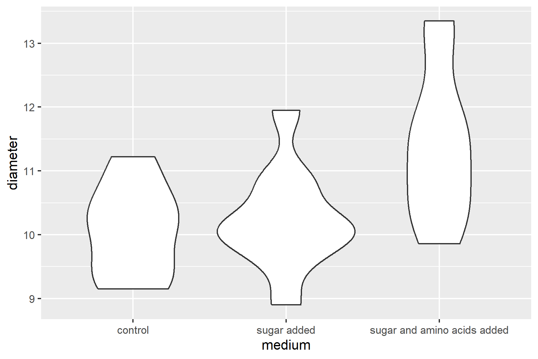

Figure 14.1: The diameters of bacterial colonies when grown in one of three media. A violin plot is a useful way to get an overview of the data and helps us identify any issues such as missing or extreme values. It also tells us what to expect from the analysis.

R will order the groups alphabetically by default.

The figure suggests that adding sugar and amino acids to the medium increases the diameter of the colonies.

Summarising the data for each medium is the next sensible step. The most useful summary statistics are the means, standard deviations, sample sizes and standard errors. I recommend the group_by() and summarise() approach:

culture_summary <- culture %>%
  group_by(medium) %>%
  summarise(mean = mean(diameter),
            std = sd(diameter),
            n = length(diameter),
            se = std/sqrt(n))

We have save the results to culture_summary so that we can use the means and standard errors in our plot later.

culture_summary
## # A tibble: 3 × 5
##   medium                       mean   std     n    se
##   <chr>                       <dbl> <dbl> <int> <dbl>
## 1 control                      10.1 0.716    10 0.226
## 2 sugar added                  10.2 0.818    10 0.259
## 3 sugar and amino acids added  11.4 1.18     10 0.373

14.3.2 Apply lm()

We can create a one-way ANOVA model like this:

mod <- lm(data = culture, diameter ~ medium)

And examine the model with:

summary(mod)
## 
## Call:
## lm(formula = diameter ~ medium, data = culture)
## 
## Residuals:
##    Min     1Q Median     3Q    Max 
## -1.541 -0.700 -0.080  0.424  1.949 
## 
## Coefficients:
##                                   Estimate Std. Error t value Pr(>|t|)    
## (Intercept)                        10.0700     0.2930  34.370  < 2e-16 ***
## mediumsugar added                   0.1700     0.4143   0.410  0.68483    
## mediumsugar and amino acids added   1.3310     0.4143   3.212  0.00339 ** 
## ---
## Signif. codes:  0 '***' 0.001 '**' 0.01 '*' 0.05 '.' 0.1 ' ' 1
## 
## Residual standard error: 0.9265 on 27 degrees of freedom
## Multiple R-squared:  0.3117, Adjusted R-squared:  0.2607 
## F-statistic: 6.113 on 2 and 27 DF,  p-value: 0.00646

The Estimates in the Coefficients table give:

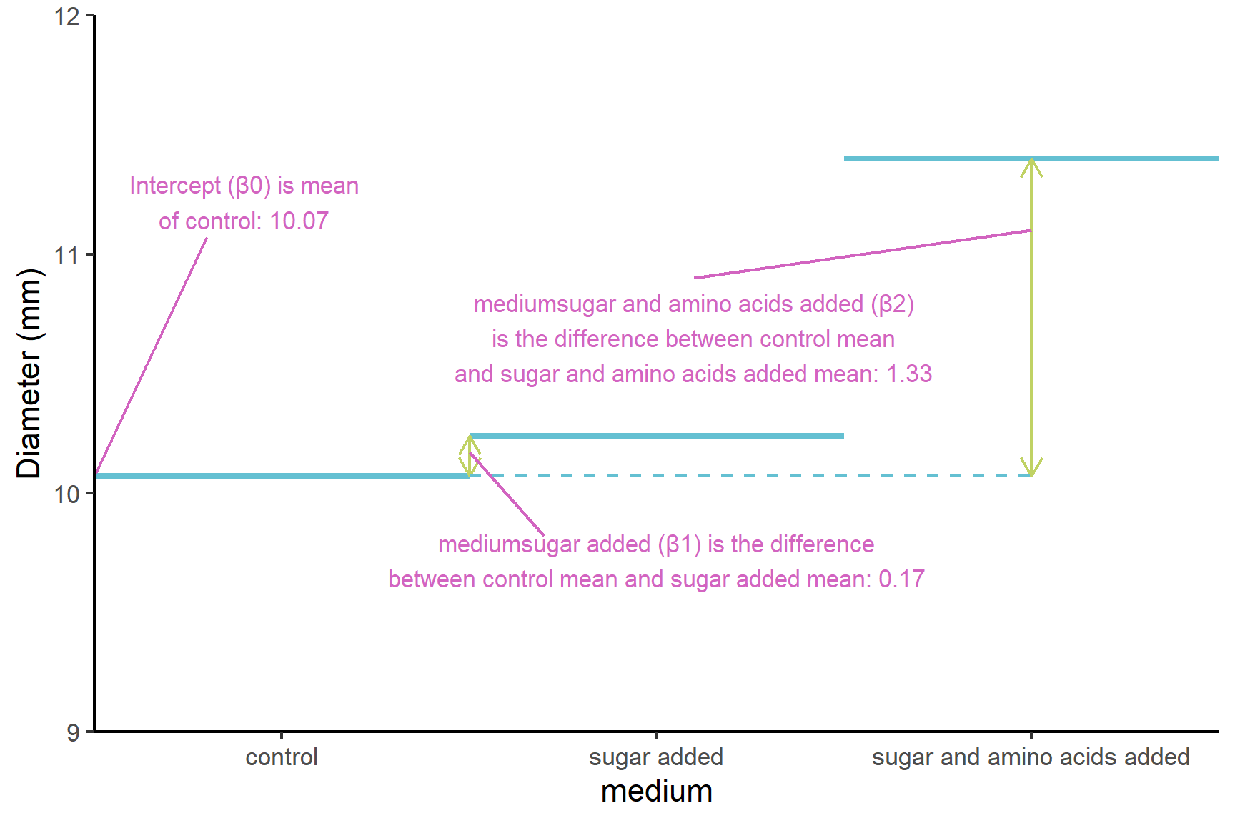
• (Intercept) known as \(\beta_0\). The mean of the control group (Figure 14.2). Just as the intercept is the value of the y (the response) when the value of x (the explanatory) is zero in a simple linear regression, this is the value of diameter when the medium is at its first level. The order of the levels is alphabetical by default.

• mediumsugar added known as \(\beta_1\). This is what needs to be added to the mean of the control group to get the mean of the ‘medium sugar added’ group (Figure 13.3). Just as the slope is amount of y that needs to be added for each unit of x in a simple linear regression, this is the amount of diameter that needs to be added when the medium goes from its first level to its second level (i.e., one unit). The mediumsugar added estimate is positive so the the ‘medium sugar added’ group mean is higher than the control group mean

• mediumsugar and amino acids added known as \(\beta_2\) is what needs to be added to the mean of the control group to get the mean of the ‘medium sugar and amino acids added’ group (Figure 13.3). Note that it is the amount added to the intercept (the control in this case). The mediumsugar and amino acids added estimate is positive so the the ‘medium sugar and amino acids added’ group mean is higher than the control group mean

If we had more groups, we would have more estimates and all would be compared to the control group mean.

The p-values on each line are tests of whether that coefficient is different from zero.

• (Intercept) 10.0700 0.2930 34.370 < 2e-16 *** tells us that the control group mean is significantly different from zero. This is not a very interesting, it just means the control colonies have a diameter.
• mediumsugar added 0.1700 0.4143 0.410 0.68483 tells us that the ‘medium sugar added’ group mean is not significantly different from the control group mean.
• mediumsugar and amino acids added 1.3310 0.4143 3.212 0.00339 ** tells us that the ‘medium sugar and amino acids added’ group mean is significantly different from the control group mean.

Note: none of this output tells us whether the medium sugar and amino acids added’ group mean is significantly different from the ‘medium sugar added’ group mean. We need to do a post-hoc test for that.

The F value and p-value in the last line are a test of whether the model as a whole explains a significant amount of variation in the response variable.

Figure 14.2: In an one-way ANOVA model with three groups, the first estimate is the intercept which is the mean of the first group. The second estimate is the ‘slope’ which is what has to added to the intercept to get the second group mean. The third estimate is the ‘slope’ which is what has to added to the intercept to get the third group mean. Note that y axis starts at 15 to create more space for the annotations.

The ANOVA is significant but this only tells us that growth medium matters, meaning at least two of the means differ. To find out which means differ, we need a post-hoc test. A post-hoc (“after this”) test is done after a significant ANOVA test. There are several possible post-hoc tests and we will be using Tukey’s HSD (honestly significant difference) test (Tukey 1949) implemented in the emmeans (Lenth 2023) package.

We need to load the package:

library(emmeans)

Then carry out the post-hoc test:

emmeans(mod, ~ medium) |> pairs()
##  contrast                                  estimate    SE df t.ratio p.value
##  control - sugar added                        -0.17 0.414 27  -0.410  0.9117
##  control - sugar and amino acids added        -1.33 0.414 27  -3.212  0.0092
##  sugar added - sugar and amino acids added    -1.16 0.414 27  -2.802  0.0244
## 
## P value adjustment: tukey method for comparing a family of 3 estimates

Each row is a comparison between the two means in the ‘contrast’ column. The ‘estimate’ column is the difference between those means and the ‘p.value’ indicates whether that difference is significant.

A plot can be used to visualise the result of the post-hoc which can be especially useful when there are very many comparisons.

emmeans(mod, ~ medium) |> plot()

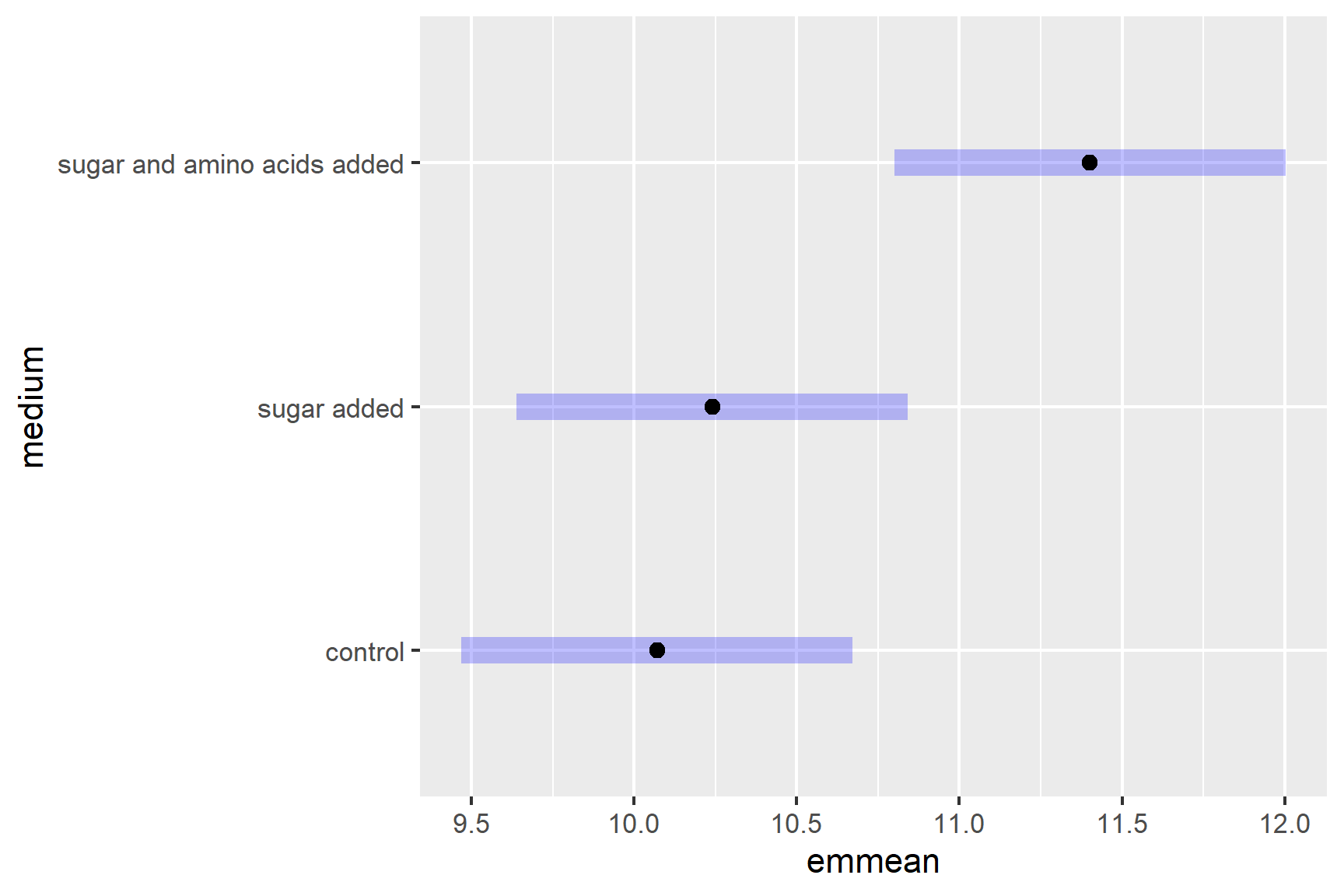
Where the purple bars overlap, there is no significant difference.

We have found that colony diameters are significantly greater when sugar and amino acids are added but that adding sugar alone does not significantly increase colony diameter.

14.3.3 Check assumptions

Check the assumptions: All general linear models assume the “residuals” are normally distributed and have “homogeneity” of variance.

Our first check of these assumptions is to use common sense: diameter is a continuous and we would expect it to be normally distributed thus we would expect the residuals to be normally distributed thus we would expect the residuals to be normally distributed

We then proceed by plotting residuals. The plot() function can be used to plot the residuals against the fitted values (See Figure 14.3). This is a good way to check for homogeneity of variance.

plot(mod, which = 1)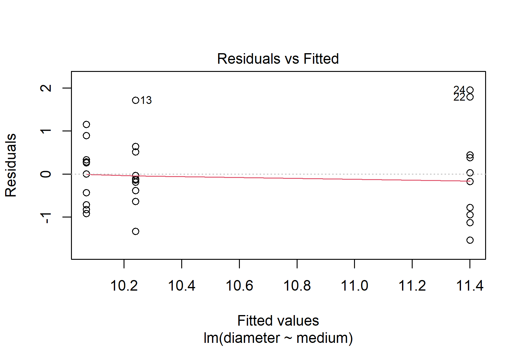

Figure 14.3: A plot of the residuals against the fitted values shows whether the points are distributed similarly in each group. Any difference seems small but perhaps the residuals are more variable for the highest mean.

Perhaps the variance is higher for the highest mean?

We can also use a histogram to check for normality (See Figure 14.4).

ggplot(mapping = aes(x = mod$residuals)) + 
  geom_histogram(bins = 8)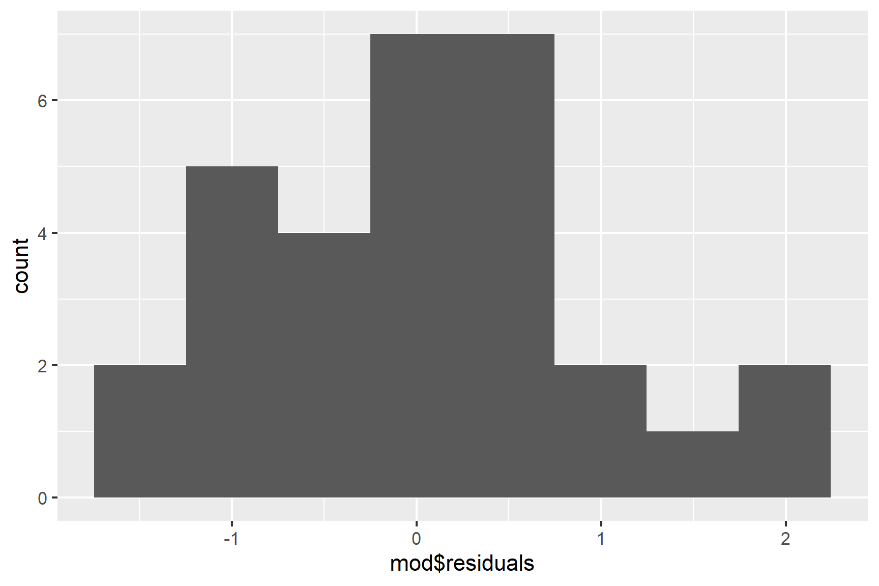

Figure 14.4: A histogram of residuals is symetrical and seems consistent with a normal distribution. This is a good sign for the assumption of normally distributed residuals.

Finally, we can use the Shapiro-Wilk test to test for normality.

shapiro.test(mod$residuals)
## 
##  Shapiro-Wilk normality test
## 
## data:  mod$residuals
## W = 0.96423, p-value = 0.3953

The p-value is greater than 0.05 so this test of the normality assumption is not significant.

Taken together, these results suggest that the assumptions of normality and homogeneity of variance are probably not violated.

14.3.4 Report

There was a significant effect of media on the diameter of bacterial colonies (F = 6.11; d.f. = 2, 27; p = 0.006). Post-hoc testing with Tukey’s Honestly Significant Difference test (Tukey 1949) revealed the colony diameters were significantly larger when grown with both sugar and amino acids (\(\bar{x} \pm s.e\): 11.4 \(\pm\) 0.37 mm) than with neither (10.2 \(\pm\) 0.26 mm; p = 0.0092) or just sugar (10.1 \(\pm\) 0.23 mm; p = 0.0244). See Figure 14.5.

ggplot() +
  geom_point(data = culture, aes(x = medium, y = diameter),
             position = position_jitter(width = 0.1, height = 0),
             colour = "gray50") +
  geom_errorbar(data = culture_summary, 
                aes(x = medium, ymin = mean - se, ymax = mean + se),
                width = 0.3) +
  geom_errorbar(data = culture_summary, 
                aes(x = medium, ymin = mean, ymax = mean),
                width = 0.2) +
  scale_y_continuous(name = "Diameter (mm)", 
                     limits = c(0, 16.5), 
                     expand = c(0, 0)) +
  scale_x_discrete(name = "Medium", 
                   labels = c("Control", 
                              "Sugar added", 
                              "Sugar and amino acids added")) +
  annotate("segment", x = 2, xend = 3, 
           y = 14, yend = 14,
           colour = "black") +
  annotate("text", x = 2.5,  y = 14.5, 
           label = expression(italic(p)~"= 0.0244")) +
    annotate("segment", x = 1, xend = 3, 
           y = 15.5, yend = 15.5,
           colour = "black") +
  annotate("text", x = 2,  y = 16, 
           label = expression(italic(p)~"= 0.0092")) +
  theme_classic()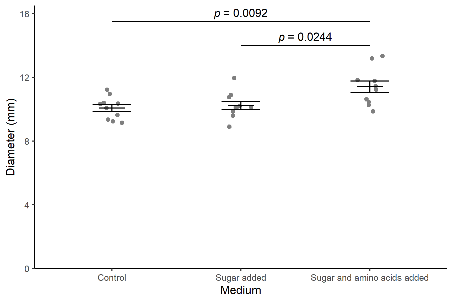

Figure 14.5: Medium affects bacterial colony diameter. Ten replicate colonies were grown on three types of media: control, with sugar added and with both sugar and amino acids added. Error bars are means \(\pm\) 1 standard error. There was a significant effect of media on the diameter of bacterial colonies (F = 6.11; d.f. = 2, 27; p = 0.006). Post-hoc testing with Tukey’s Honestly Significant Difference test (Tukey 1949) revealed the colony diameters were significantly larger when grown with both sugar and amino acids than with neither or just sugar. Data analysis was conducted in R (R Core Team 2023) with tidyverse packages (Wickham et al. 2019).

15 Kruskal-Wallis

Our examination of the assumptions revealed a possible violation of the assumption of homogeneity of variance. We might reasonably apply a non-parametric test to this data.

The Kruskal-Wallis (Kruskal and Wallis 1952) is non-parametric equivalent of a one-way ANOVA. The general question you have about your data - do these groups differ (or does the medium effect diameter) - is the same, but one of more of the following is true:

• the response variable is not continuous
• the residuals are not normally distributed
• the sample size is too small to tell if they are normally distributed.
• the variance is not homogeneous

Summarising the data using the median and interquartile range is more aligned to the type of analysis than using means and standard deviations:

culture_summary <- culture |> 
  group_by(medium) |> 
  summarise(median = median(diameter),
            interquartile  = IQR(diameter),
            n = length(diameter))

View the results:

culture_summary
## # A tibble: 3 × 4
##   medium                      median interquartile     n
##   <chr>                        <dbl>         <dbl> <int>
## 1 control                       10.2         0.968    10
## 2 sugar added                   10.1         0.713    10
## 3 sugar and amino acids added   11.3         1.33     10

15.0.1 Apply kruskal.test()

We pass the dataframe and variables to kruskal.test() in the same way as we did for lm(). We give the data argument and a “formula” which says diameter ~ medium meaning “explain diameter by medium”.

kruskal.test(data = culture, diameter ~ medium)
## 
##  Kruskal-Wallis rank sum test
## 
## data:  diameter by medium
## Kruskal-Wallis chi-squared = 8.1005, df = 2, p-value = 0.01742

The result of the test is given on this line: Kruskal-Wallis chi-squared = 8.1005, df = 2, p-value = 0.01742. Chi-squared is the test statistic. The p-value is less than 0.05 meaning there is a significant effect of medium on diameter.

Notice that the p-value is a little larger than for the ANOVA. This is because non-parametric tests are generally more conservative (less powerful) than their parametric equivalents.

A significant Kruskal-Wallis tells us at least two of the groups differ but where do the differences lie? The Dunn test (Dunn 1964) is a post-hoc multiple comparison test for a significant Kruskal-Wallis. It is available in the package FSA (Ogle et al. 2023)

Load the package using:

library(FSA)

Then run the post-hoc test with:

dunnTest(data = culture, diameter ~ medium)
##                                  Comparison          Z    P.unadj      P.adj
## 1                     control - sugar added -0.2159242 0.82904681 0.82904681
## 2     control - sugar and amino acids added -2.5656880 0.01029714 0.03089142
## 3 sugar added - sugar and amino acids added -2.3497637 0.01878533 0.03757066

The P.adj column gives p-value for the comparison listed in the first column. Z is the test statistic. The p-values are a little larger for the control - sugar and amino acids added comparison and the sugar added - sugar and amino acids added comparison but they are still less than 0.05. This means our conclusions are the same as for the ANOVA.

15.0.2 Report

There is a significant effect of media on the diameter of bacterial colonies (Kruskal-Wallis: chi-squared = 6.34; df = 2; p-value = 0.042) with colonies growing significantly better when both sugar and amino acids are added to the medium. Post-hoc testing with the Dunn test (Dunn 1964) revealed the colony diameters were significantly larger when grown with both sugar and amino acids (median = 11.3 mm) than with neither (median = 10.2 mm; p = 0.031) or just sugar (median = 10.2 mm; p = 0.038). See Figure 15.1.

ggplot(data = culture, aes(x = medium, y = diameter)) +
 geom_boxplot() +
  scale_y_continuous(name = "Diameter (mm)", 
                     limits = c(0, 16.5), 
                     expand = c(0, 0)) +
  scale_x_discrete(name = "Medium", 
                   labels = c("Control", 
                              "Sugar added", 
                              "Sugar and amino acids added")) +
  annotate("segment", x = 2, xend = 3, 
           y = 14, yend = 14,
           colour = "black") +
  annotate("text", x = 2.5,  y = 14.5, 
           label = expression(italic(p)~"= 0.038")) +
    annotate("segment", x = 1, xend = 3, 
           y = 15.5, yend = 15.5,
           colour = "black") +
  annotate("text", x = 2,  y = 16, 
           label = expression(italic(p)~"= 0.031")) +
  theme_classic()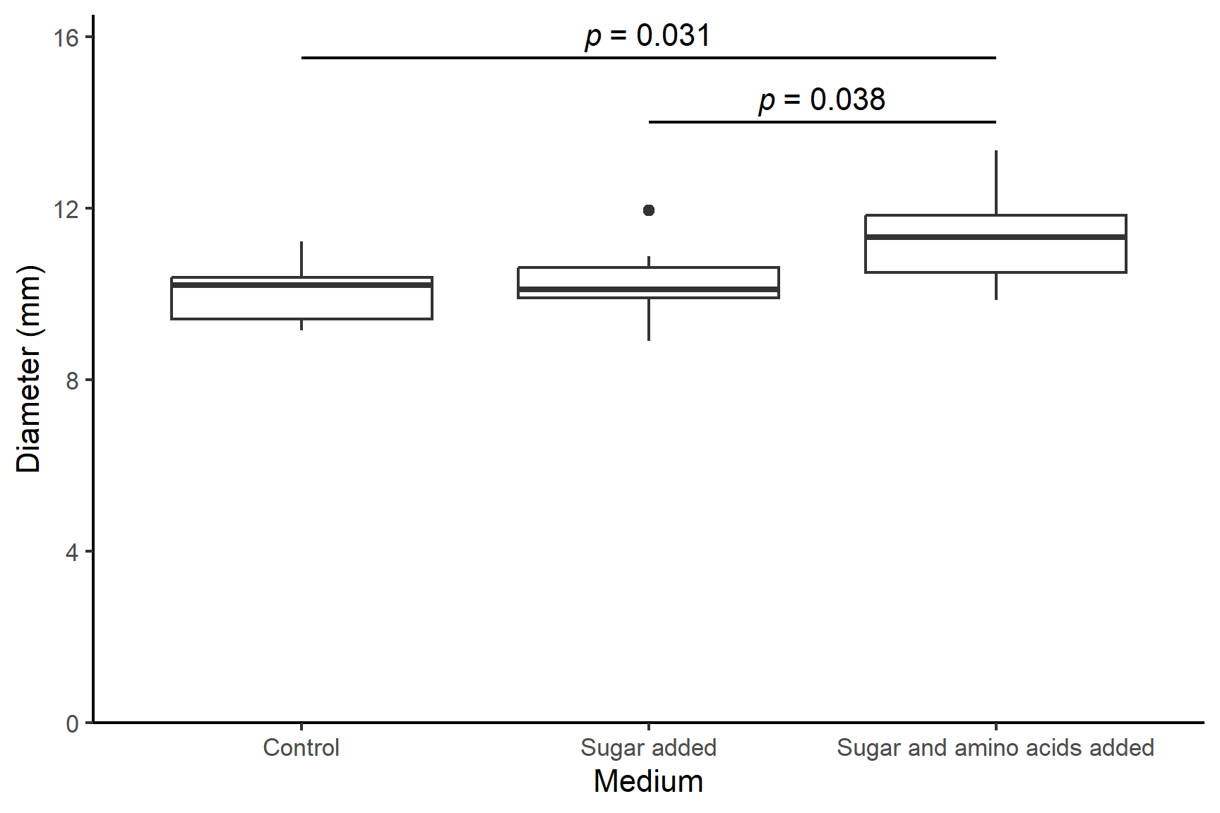

Figure 15.1: Medium affects bacterial colony diameter. Ten replicate colonies were grown on three types of media: control, with sugar added and with both sugar and amino acids added. The heavy lines indicate median diameter, boxes indicate the interquartile range and whiskers the range. There was a significant effect of media on the diameter of bacterial colonies (Kruskal-Wallis: chi-squared = 6.34, df = 2, p-value = 0.042). Post-hoc testing with the Dunn test (Dunn 1964) revealed the colony diameters were significantly larger when grown with both sugar and amino acids than with neither or just sugar. Data analysis was conducted in R (R Core Team 2023) with tidyverse packages (Wickham et al. 2019).

16 Summary

1. A linear model with one explanatory variable with two or more groups is also known as a one-way ANOVA.

2. We estimate the coefficients (also called the parameters) of the model. For a one-way ANOVA with three groups these are the mean of the first group, \(\beta_0\), the difference between the means of the first and second groups, \(\beta_1\), and the difference between the means of the first and third groups, \(\beta_2\). We test whether the parameters differ significantly from zero

3. We can use lm() to one-way ANOVA in R.

4. In the output of lm() the coefficients are listed in a table in the Estimates column. The p-value for each coefficient is in the test of whether it differs from zero. At the bottom of the output there is an \(F\) test of the model overall. Now we have more than two parameters, this is different from the test on any one parameter. The R-squared value is the proportion of the variance in the response variable that is explained by the model. It tells us is the explanatory variable is useful in predicting the response variable overall.

5. When the \(F\) test is significant there is a significant effect of the explanatory variable on the response variable. To find out which means differ, we need a post-hoc test. Here we use Tukey’s HSD applied with the emmeans() and pairs() functions from the emmeans package. Post-hoc tests make adjustments to the p-values to account for the fact that we are doing multiple tests.

6. The assumptions of the general linear model are that the residuals are normally distributed and have homogeneity of variance. A residual is the difference between the predicted value and the observed value.

7. We examine a histogram of the residuals and use the Shapiro-Wilk normality test to check the normality assumption. We check the variance of the residuals is the same for all fitted values with a residuals vs fitted plot.

8. If the assumptions are not met, we can use the Kruskal-Wallis test applied with kruskal.test() in R and follow it with The Dunn test applied with dunnTest() in the package FSA.

9. When reporting the results of a test we give the significance, direction and size of the effect. Our figures and the values we give should reflect the type of test we have used. We use means and standard errors for parametric tests and medians and interquartile ranges for non-parametric tests. We also give the test statistic, the degrees of freedom (parametric) or sample size (non-parametric) and the p-value. We annotate our figures with the p-value, making clear which comparison it applies to.

Dunn, Olive Jean. 1964. “Multiple Comparisons Using Rank Sums.” Technometrics 6 (3): 241–52. https://doi.org/10.1080/00401706.1964.10490181.

Kruskal, William H., and W. Allen Wallis. 1952. “Use of Ranks in One-Criterion Variance Analysis.” Journal of the American Statistical Association 47 (260): 583–621. https://doi.org/10.1080/01621459.1952.10483441.

Lenth, Russell V. 2023. “Emmeans: Estimated Marginal Means, Aka Least-Squares Means.” https://CRAN.R-project.org/package=emmeans.

Ogle, Derek H., Jason C. Doll, A. Powell Wheeler, and Alexis Dinno. 2023. “FSA: Simple Fisheries Stock Assessment Methods.” https://CRAN.R-project.org/package=FSA.

R Core Team. 2023. R: A Language and Environment for Statistical Computing. Vienna, Austria: R Foundation for Statistical Computing. https://www.R-project.org/.

Tukey, John W. 1949. “Comparing Individual Means in the Analysis of Variance.” Biometrics 5 (2): 99–114. https://doi.org/10.2307/3001913.

Wickham, Hadley. 2014. “Tidy Data.” Journal of Statistical Software, Articles 59 (10): 1–23. https://vita.had.co.nz/papers/tidy-data.pdf.

Wickham, Hadley, Mara Averick, Jennifer Bryan, Winston Chang, Lucy D’Agostino McGowan, Romain François, Garrett Grolemund, et al. 2019. “Welcome to the Tidyverse” 4: 1686. https://doi.org/10.21105/joss.01686.