19  Finding the molecular weight of proteins migrated on a western blot

Incomplete

You are reading a work in progress. This page is a dumping ground for ideas. Sections maybe missing, or contain a list of points to include.

19.1 What is a Western Blot?

A Western blot is a laboratory technique used to detect specific proteins in a sample. Proteins are isolated from the sample, sorted by size using SDS-PAGE and then transferred to a membrane (usually nitrocellulose or PVDF). The membrane is incubated with a primary antibody that binds to the target protein. A secondary antibody, linked to a detectable enzyme or fluorophore, binds to the primary antibody so the protein of interested can be detected. The result is a band on the membrane. The molecular weight of a protein can be estimated from the position of the band on the membrane because the distance travelled by the protein is inversely proportional to the log of the molecular weight. The intensity of the band can also be used to estimate the amount of protein present in the sample.

19.2 Scenario

Macrophages are immune cells that play a key role in the body’s defense against pathogens. They can be activated by various stimuli, including bacterial infection. In this experiment, we are interested in the production of TNF-alpha, a pro-inflammatory cytokine, in response to bacterial infection. We will use a Western blot to determine the

Macrophages are treated with one of three treatments: Media, LPS or NeonGreen fluorescent E.coli Macrophages produce TNF-α in response to bacterial infection

Model western blot data containing protein weight markers (lane 1) and anti-TNFalpha stained samples for media (in lane 2), LPS-stimulated (in lane 3), and E.coli-stimulated (in lane 4) samples.

A picture of the protein weight markers used in the experiments with their associated weights in kilodaltons (kDa).

library(tidyverse)
library(imager)

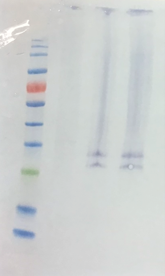
Use the imager package to import your Western blot image.

blot <- load.image("data-images/western-blot-anti-TNFalpha stained-macrophages.png")

plot(blot)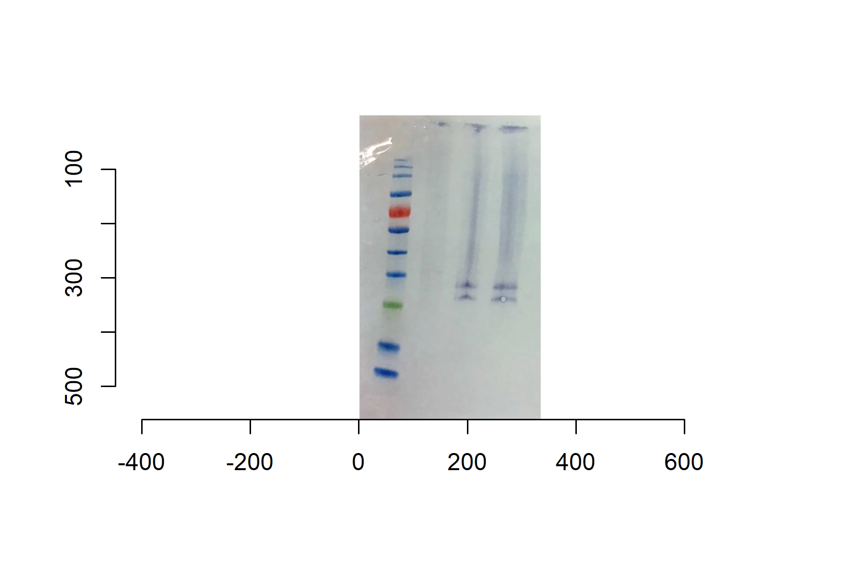

For a typical blot, y increases downwards, so smaller bands (higher kDa) are higher up.

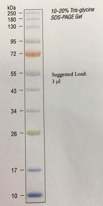
Annotate the Lanes and Marker Lane

# Number of bands in your marker lane
# click from the top or gel to the bottom 
# i.e., high MW to low
marker_positions <- locator(n = 11)  

# make sure these are in the same order 
# that you clicked lanes in
# i.e., high MW to low

marker_df <- tibble(
  x = marker_positions$x,
  y = marker_positions$y,
  # Replace with your actual marker weights
  KDa = c(250, 180, 130, 95, 72, 55, 43, 34, 26, 17, 10)  
)

migration_points <- locator(n = 2)

origin_y <- migration_points$y[1]
front_y <- migration_points$y[2]
total_migration <- abs(front_y - origin_y)

# band positions for each sample: LPS, E.coli
tnf_positions <- locator(n = 2)  

tnf_df <- tibble(
  x = tnf_positions$x,
  y = tnf_positions$y,
  distance_migrated = abs(tnf_positions$y - origin_y),
  Rf = distance_migrated / total_migration
)

marker_df <- marker_df  |> 
  mutate(
    distance_migrated = abs(y - origin_y),
    Rf = distance_migrated / total_migration,
    log_kda = log10(KDa)
  )

ggplot(data = marker_df, aes(x = Rf, y = log_kda)) +
  geom_point() +
  geom_smooth(method = "lm", se = FALSE)

model <- lm(log_kda ~ Rf, data = marker_df)
summary(model)

# Predict TNF band molecular weight
tnf_df <- tnf_df  |> 
  mutate(
    predicted_log_kda = predict(model, newdata = tnf_df),
    predicted_kda = 10^predicted_log_kda
  )

TNF-alpha has a molecular weight of approximately 17 kDa for the monomeric form and 52 kDa for the homotrimer. The 17 kDa monomer is often observed on SDS-PAGE under reducing conditions, while the trimer is the form typically secreted. The predicted molecular weight of the precursor membrane-bound form is around 26 kDa.

Thus, we have the precursor membrane-bound form.

ggplot(data = marker_df, aes(x = Rf, y = log_kda)) +
  geom_point(size = 2) +
  geom_smooth(method = "lm", 
              se = FALSE,
              colour = "black",
              linetype = 2) +
   geom_point(data = tnf_df, 
              aes(x = Rf, y = predicted_log_kda), 
              shape = 23, size = 3) +
  theme_classic()

plot(blot, axes = FALSE)
points(marker_df$x, marker_df$y, pch = "--")
text(20, 
     marker_df$y, labels = marker_df$KDa, cex = 0.8)
text(c(140, 210, 275), 
     c(10,10, 10), labels = c("Media"), cex = 0.8)