qnorm(0.975)
## [1] 1.95996410 Confidence Intervals
Just needs proof reading
You are reading a work in progress. This page is compete but needs final proof reading.
10.1 What is a confidence interval?
When we calculate a mean from a sample, we are using it to estimate the mean of the population. Confidence intervals are a range of values and are a way to quantify the uncertainty in our estimate. When we report a mean with its 95% confidence interval we give the mean plus and minus some variation. We are saying that 95% of the time, that range will contain the population mean.
The confidence interval is calculated from the sample mean and the standard error of the mean. The standard error of the mean is the standard deviation of the sampling distribution of the mean.
To understand confidence intervals we need to understand some properties of the normal distribution.
10.2 The normal distribution
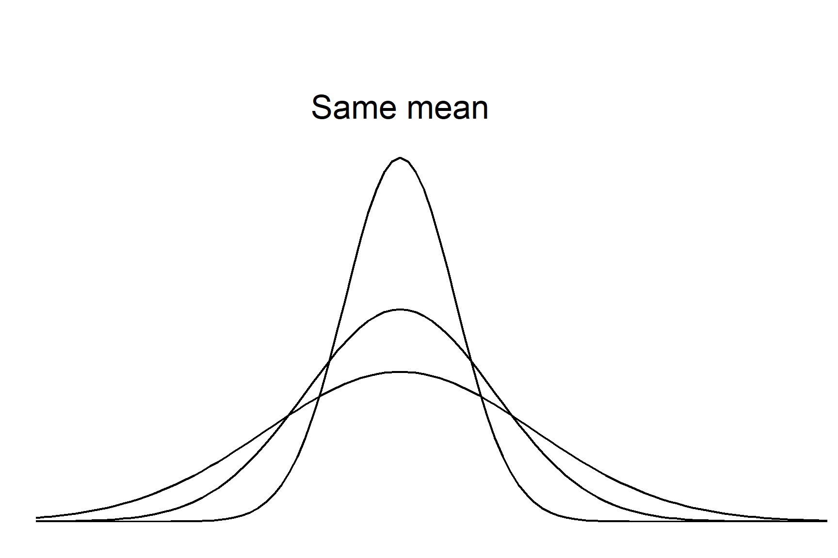
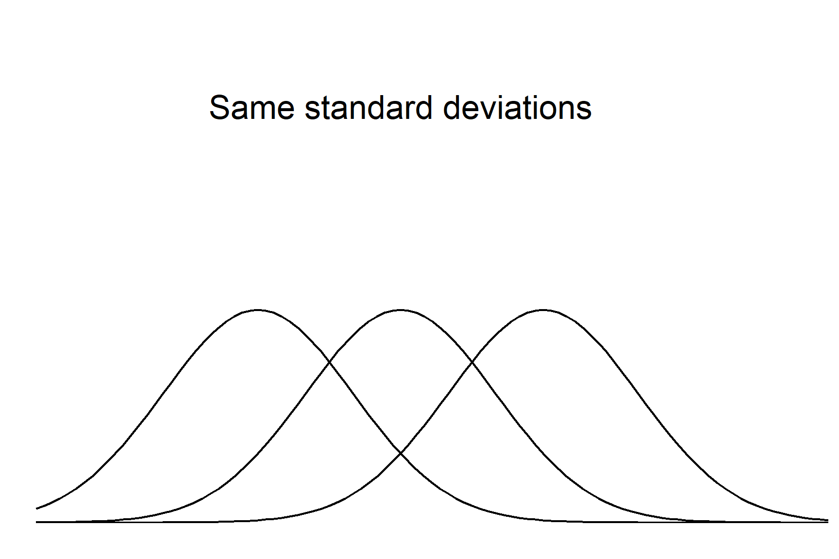
A distribution describes the values the variable can take and the chance of them occurring. A distribution has a general type, given by the function, and is further tuned by the parameters in the function. For the normal distribution these parameters are the mean and the standard deviation. Every variable that follows the normal distribution has the same bell shaped curve and the distributions differ only in their means and/or standard deviations. The mean determines where the centre of the distribution is, the standard deviation determines the spread (Figure 10.1).
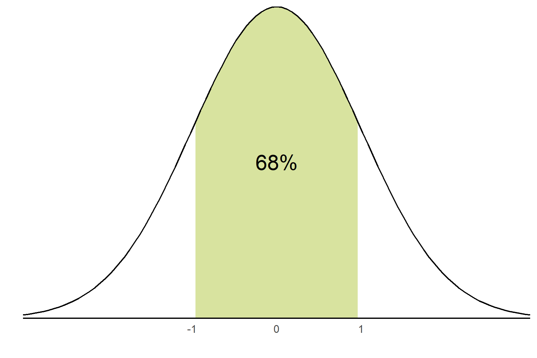
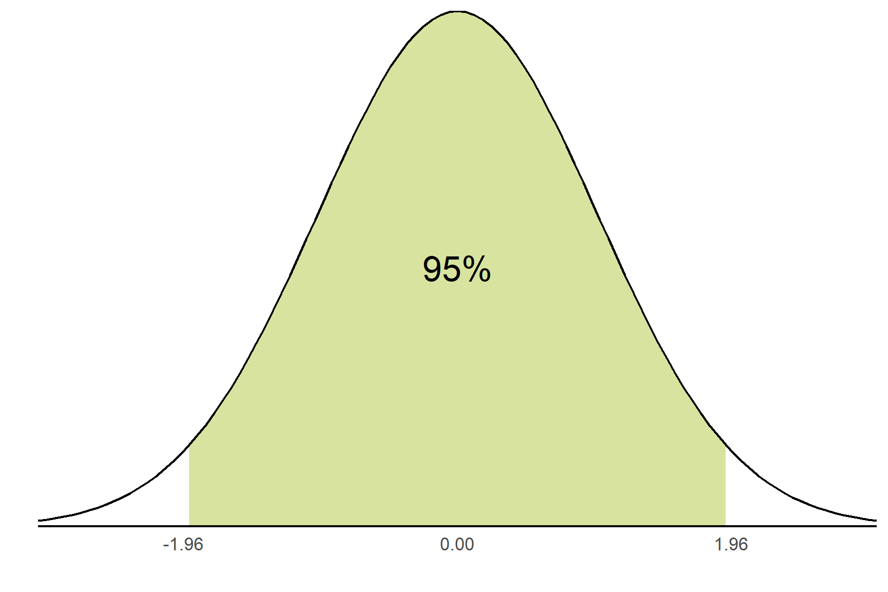
Whilst normal distributions vary in the location on the horizontal axis and their width, they all share some properties and it is these shared properties that allow the calculation of confidence intervals with some standard formulae. The properties are that a fix percentage of values lie between a given number of standard deviations. For example, 68.2% values lie between plus and minus one standard deviation from the mean and 95% values lie between \(\pm\) 1.96 standard deviations. Another way of saying this is that there is a 95% chance that a randomly selected value will lie between \(\pm\) 1.96 standard deviations from the mean. This is illustrated in Figure 10.2.
R has some useful functions associated with distributions, including the normal distribution.
10.2.1 Distributions: the R functions
For any distribution, R has four functions:
- the density function, which gives the height of the function at a given value.
- the distribution function, which gives the probability that a variable takes a particular value or less. This is the area under the curve.
- the quantile function which is the inverse of the Distribution function, i.e., it returns the value (‘quantile’) for a given probability.
- the random number generating function.
The functions are named with a letter d, p, q or r preceding the distribution name. Table 10.1 shows these four functions for some common distributions: the normal, binomial, Poisson and t distributions.
The functions which are of most use to us are those for the normal distribution: pnorm() and qnorm(). These are illustrated in Figure 10.3.
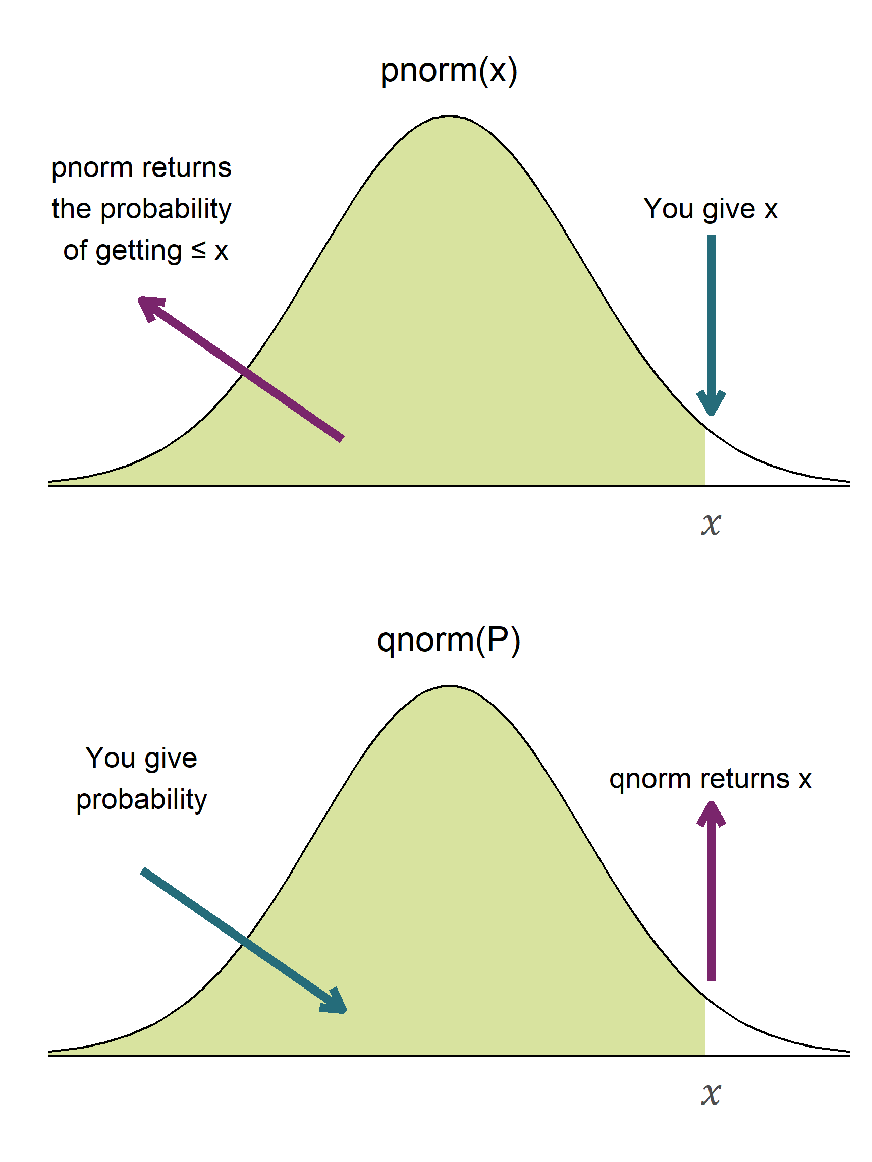
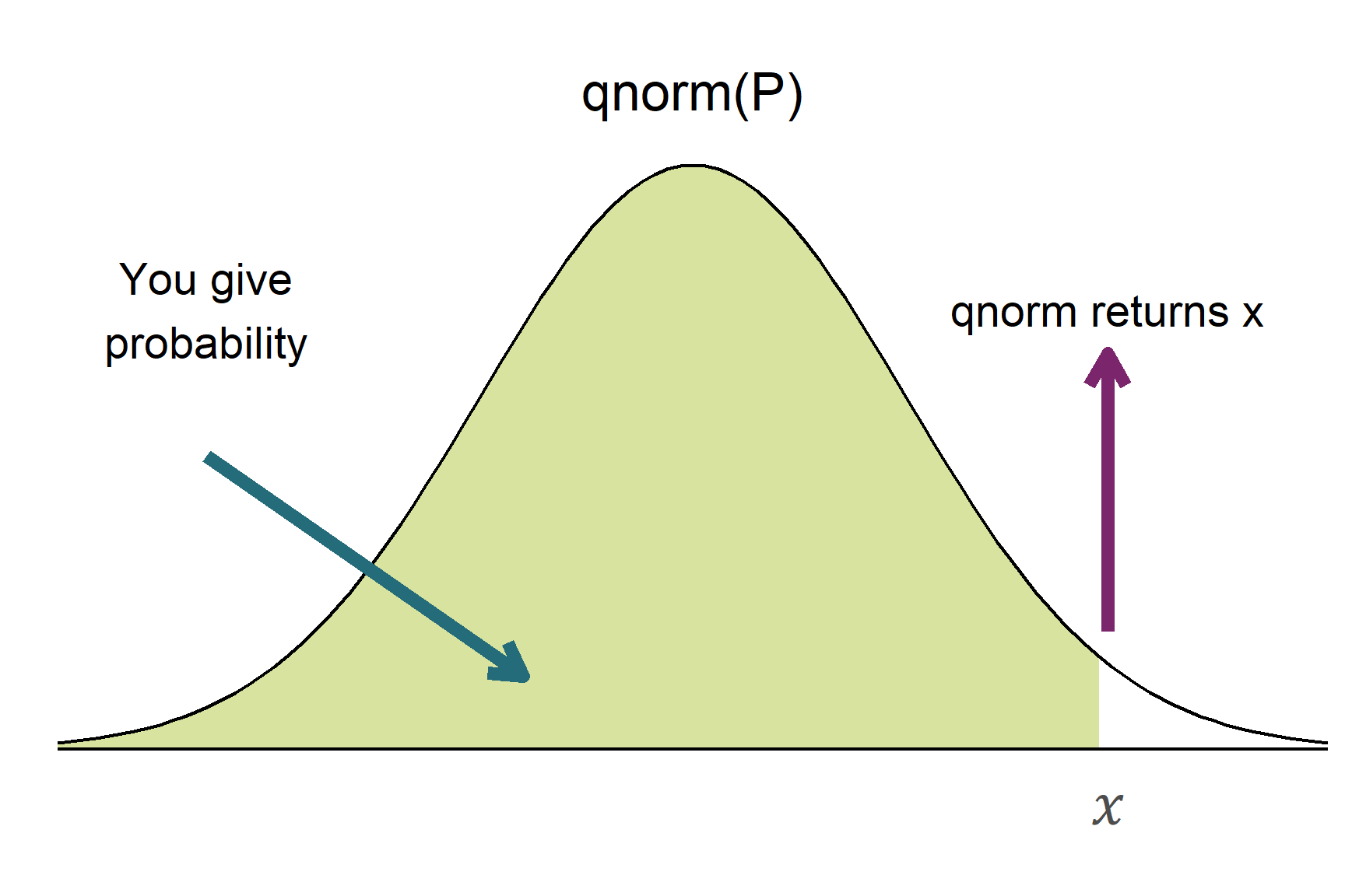
pnorm() and qnorm() functions return values related to the normal distribution. Figure 10.3 (a) pnorm() returns the probability (the area under the curve) to the right of a given x-value. Figure 10.3 (b) qnorm() returns the value along the x-axis corresponding to a given cumulative probability.
Searching for the manual with ?normal or any one of the functions (?pnorm) will bring up a single help page for all four associated functions.
dnorm(), pnorm(), qnorm() and rnorm(). The first letter of each function indicates the type of function: d for density, p for distribution, q for quantile and r for random number generator.
10.3 Confidence intervals on large samples
\[ \bar{x} \pm 1.96 \times s.e. \tag{10.1}\]
95% of confidence intervals calculated in this way will contain the true population mean.
Do you have to remember the value of 1.96? Not if you have R!
Notice that it is qnorm(0.975) and not qnorm(0.95) for a 95% confidence interval. This is because the functions are defined as giving the area under to the curve to the left of the value given. This is known as being “one-tailed”. To get 0.05 in the two tails combined, we need to have 0.025 - half of 0.05 - in each tail. The value on the x-axis that puts 0.025 in the upper tail is 0.975 (Figure 10.5). If we gave 0.95, we would get the value that put 0.05 in one tail and 0.9 in the central area. We want 0.025 in each tail, so we need to use 0.975 in qnorm().
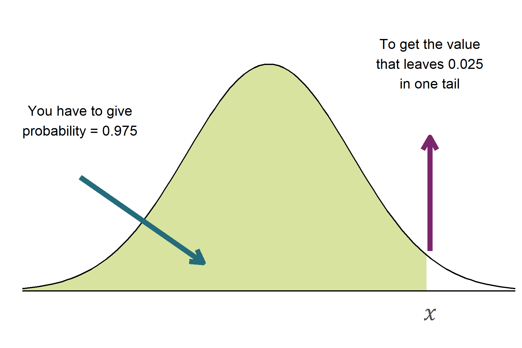
qnorm() a probability, returns the value on the x-axis below which that proportion of the distribution lies. For a confidence interval of 95%, we need the values on the x-axis that capture the middle 95% of the normal distribution. This is 0.025 in each tail.
10.4 Confidence intervals on small samples
The calculation of confidence intervals on small samples is very similar but we use the t-distribution rather than the normal distribution. The formula is:
\[ \bar{x} \pm t_{[d.f.]} \times s.e. \tag{10.2}\]
The t-distibution is a modified version of the normal distribution and we use it because the sampling distribution of the mean is not quite normal when the sample size is small. The t-distribution has an additional parameter called the degrees of freedom which is the sample size minus one (\(n -1\)). Like the normal distribution, the t-distribution has a mean of zero and is symmetrical. However, The t-distribution has fatter tails than the normal distribution and this means that the probability of getting a value in the tails is higher than for the normal distribution. The degrees of freedom determine how much fatter the tails are. The smaller the sample size, the fatter the tails. As the sample size increases, the t-distribution becomes more and more like the normal distribution.
10.4.1 What are degrees of freedom?
Degrees of freedom (usually abbreivated d.f.) describe how much independent information is available to estimate variability when calculating probabilities. In a population, all values are known, so no parameters need estimating. In a sample, we estimate parameters such as the mean. In estimating a mean, only \(n - 1\) values can vary independently because one value is constrained by the sample mean. In hypothesis tests and confidence intervals, d.f. adjust for uncertainty when generalizing from a sample to a population, affecting probability distributions like the t-distribution. More d.f. mean better probability estimates, while fewer d.f. reflect greater uncertainty in estimating population parameters.
10.5 🎬 Your turn!
If you want to code along you will need to start a new RStudio project, add a data-raw folder and open a new script. You will also need to load the tidyverse package (Wickham et al. 2019).
10.6 Large samples
A team of biomedical researchers is studying the concentration of Creatine Kinase (CK) in the blood of patients with muscle disorders. They collect a large random sample (n = 100) of blood samples from patients and measure the CK concentration in UL-1 (units per litre).
The goal is to estimate the average CK concentration in this patient population and calculate a 95% confidence interval for the mean concentration. The data are in ck_concen.csv
10.6.1 Import
creatinekinase <- read_csv("data-raw/ck_concen.csv")10.6.2 Calculate sample statistics
We can use the summarise() function to calculate: the mean, standard deviation, sample size and standard error and save t hem in a dataframe called creatine_summary
| mean | n | sd | se |
|---|---|---|---|
| 302.1687 | 100 | 90.71385 | 9.071385 |
10.6.3 Calcuate C.I.
To calculate the 95% confidence interval we need to look up the quantile (multiplier) using qnorm():
q <- qnorm(0.975)Now we can use it in our confidence interval calculation:
| mean | n | sd | se | lcl95 | ucl95 |
|---|---|---|---|---|---|
| 302.1687 | 100 | 90.71385 | 9.071385 | 284.3891 | 319.9483 |
I used the names lcl95 and ucl95 to stand for “95% lower confidence limit” and “95% upper confidence limit” respectively.
This means we are 95% confident the population mean lies between 284.39 UL-1 and 319.95 UL-1. The amount we have added/subtracted from the mean (q * se) is 17.78 thus we sometimes see this written as 302.17 \(\pm\) 17.78 mm.
10.6.4 Report
The mean creatine kinase concentration in patients with muscle disorders is 302.17 UL-1, 95% C.I. [284.39, 319.95]
10.7 Small samples
TO DO
10.8 Summary of Confidence Intervals
A confidence interval gives a range of plausible values for a population mean from a sample and is calculated from a sample mean and standard error.
They are possible because all normal distributions have the same properties.
-
95% Confidence Intervals for Large Samples:
- Formula:
\[ \bar{x} \pm 1.96 \times s.e. \] - 95% of confidence intervals computed this way will contain the true population mean.
- Formula:
-
95% Confidence Intervals for Small Samples:
- Uses the t-distribution instead of the normal distribution.
- Formula:
\[ \bar{x} \pm t_{[d.f.]} \times s.e. \] - The t-distribution has fatter tails and varies based on degrees of freedom (n-1), approaching the normal distribution as n increases.
- Uses the t-distribution instead of the normal distribution.