15  Two-way ANOVA

Just needs proof reading

You are reading a work in progress. This page is compete but needs final proof reading.

15.1 Overview

In the last chapter, we learnt how to use and interpret the general linear model when the x variable was categorical with two or more groups. This procedure is known as one-way ANOVA. We will now incorporate a second categorical variable. This is often known as the two-way or two-factor ANOVA (analysis of variance). It might also be described as a “factorial design”.

In the last chapter we conducted a one-way ANOVA to test whether there was an of media on the diameter of bacterial colonies. Suppose we had run this experiment on more than one bacterial species. We would then have two explanatory variables: media and species. Perhaps we should do two one-way ANOVAs, one for each explanatory variable? This would tell us whether each explanatory variable had an effect on the response variable. However, it would not tell us whether there was an interaction between the two variables. An interaction is when the effect of one variable depends on the level of another and in some ways it is the most interesting result we could reveal. For example, we might find that the optimal media for one species was not the optimal media for the other species. A two-way ANOVA allows us to test for the effects of each explanatory variable and whether they interact. A two-way ANOVA has three null hypotheses:

1. There is no effect of media on diameter, or there is no difference between the mean diameter of colonies grown on different media.
2. There is no effect of species on diameter, or there is no difference between bacteria in colony diameter.
3. The effect of media is the same for all species, or the effect of media does not depend on species.

As a General linear model, two-way ANOVA is a parametric test with assumptions based on the normal distribution which need to be met for the p-values generated to be accurate. We use lm() to fit the model, anova() to test the significance of the explanatory variables and emmeans() and pairs() for post-hoc testing.

15.1.1 Model assumptions

We examine the model assumptions in the same way as we did for single linear regression, two-sample tests and one-way ANOVA: we apply the general linear model with lm() and then check the assumptions using diagnostic plots and the Shapiro-Wilk normality test. We also use common sense:

• the response should be continuous (or nearly continuous, see Ideas about data: Theory and practice) and we consider whether we would expect the response to be normally distributed.
• we expect decimal places and few repeated values.

15.1.2 Reporting

In reporting the result of two-way ANOVA, we include:

1. the significance of each of the explanatory variables and the interaction between them.

   • The F-statistic and p-value for each explanatory variable and the interaction term.

2. the direction of effect - which of the means is greater

   • Post-hoc test

3. the magnitude of effect - how big is the difference between the means

   • the means and standard errors for each group

Figures should reflect what you have said in the statements. Ideally they should show both the raw data and the statistical model: means and standard errors

We will explore all of these ideas with some examples.

15.2 🎬 Your turn!

If you want to code along you will need to start a new RStudio project, add a data-raw folder and open a new script. You will also need to load the tidyverse package (Wickham et al. 2019).

15.3 Two-way ANOVA

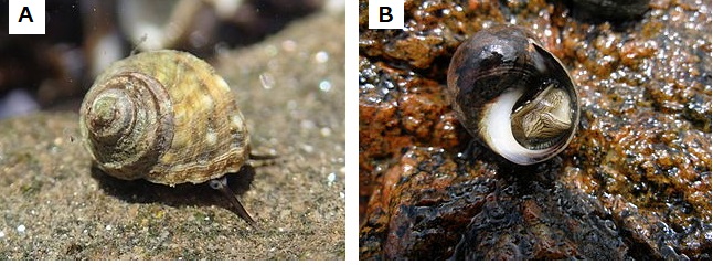
Researchers have collected live specimens of two species of periwinkle (See Figure 15.1) from sites in northern England in the Spring and Summer. They took a measure of the gut parasite load by examining a slide of gut contents. The data are in periwinkle.txt. The data were collected to determine whether there was an effect of season or species on parasite load and whether these effects were independent.

Figure 15.1: Periwinkles are marine gastropod molluscs (slugs and snails). A) Littorina brevicula (PD files - Public Domain, https://commons.wikimedia.org/w/index.php?curid=30577419) B) Littorina littorea. (photographed by Guttorm Flatabø (user:dittaeva). - Photograph taken with an Olympus Camedia C-70 Zoom digital camera. Metainformation edited with Irfanview, possibly cropped with jpegcrop., CC BY-SA 3.0, https://commons.wikimedia.org/w/index.php?curid=324769

15.3.1 Import and explore

Import the data:

periwinkle <- read_delim("data-raw/periwinkle.txt", delim = "\t")

para	season	species
58.86	Spring	Littorina brevicula
51.73	Spring	Littorina brevicula
54.99	Spring	Littorina brevicula
39.84	Spring	Littorina brevicula
65.05	Spring	Littorina brevicula
67.46	Spring	Littorina brevicula
60.38	Spring	Littorina brevicula
54.42	Spring	Littorina brevicula
47.71	Spring	Littorina brevicula
66.87	Spring	Littorina brevicula
51.02	Spring	Littorina brevicula
43.95	Spring	Littorina brevicula
62.40	Spring	Littorina brevicula
55.67	Spring	Littorina brevicula
58.45	Spring	Littorina brevicula
43.52	Spring	Littorina brevicula
69.29	Spring	Littorina brevicula
71.22	Spring	Littorina brevicula
64.60	Spring	Littorina brevicula
58.53	Spring	Littorina brevicula
51.15	Spring	Littorina brevicula
70.62	Spring	Littorina brevicula
55.10	Spring	Littorina brevicula
47.00	Spring	Littorina brevicula
54.48	Spring	Littorina brevicula
43.52	Spring	Littorina littorea
63.26	Spring	Littorina littorea
58.76	Spring	Littorina littorea
61.38	Spring	Littorina littorea
63.70	Spring	Littorina littorea
45.69	Spring	Littorina littorea
45.20	Spring	Littorina littorea
77.23	Spring	Littorina littorea
57.12	Spring	Littorina littorea
49.32	Spring	Littorina littorea
72.92	Spring	Littorina littorea
47.95	Spring	Littorina littorea
78.70	Spring	Littorina littorea
77.01	Spring	Littorina littorea
71.70	Spring	Littorina littorea
69.36	Spring	Littorina littorea
66.46	Spring	Littorina littorea
76.35	Spring	Littorina littorea
75.55	Spring	Littorina littorea
54.59	Spring	Littorina littorea
62.02	Spring	Littorina littorea
58.50	Spring	Littorina littorea
76.09	Spring	Littorina littorea
68.85	Spring	Littorina littorea
84.55	Spring	Littorina littorea
61.60	Summer	Littorina brevicula
70.84	Summer	Littorina brevicula
68.89	Summer	Littorina brevicula
67.68	Summer	Littorina brevicula
88.68	Summer	Littorina brevicula
64.64	Summer	Littorina brevicula
69.71	Summer	Littorina brevicula
70.65	Summer	Littorina brevicula
56.85	Summer	Littorina brevicula
80.06	Summer	Littorina brevicula
80.93	Summer	Littorina brevicula
53.62	Summer	Littorina brevicula
56.77	Summer	Littorina brevicula
101.81	Summer	Littorina brevicula
81.65	Summer	Littorina brevicula
88.73	Summer	Littorina brevicula
67.50	Summer	Littorina brevicula
73.75	Summer	Littorina brevicula
75.80	Summer	Littorina brevicula
74.70	Summer	Littorina brevicula
68.26	Summer	Littorina brevicula
89.29	Summer	Littorina brevicula
75.09	Summer	Littorina brevicula
74.99	Summer	Littorina brevicula
76.03	Summer	Littorina brevicula
66.67	Summer	Littorina littorea
61.31	Summer	Littorina littorea
51.00	Summer	Littorina littorea
67.43	Summer	Littorina littorea
78.12	Summer	Littorina littorea
79.26	Summer	Littorina littorea
69.03	Summer	Littorina littorea
76.14	Summer	Littorina littorea
86.81	Summer	Littorina littorea
97.56	Summer	Littorina littorea
64.64	Summer	Littorina littorea
68.64	Summer	Littorina littorea
65.95	Summer	Littorina littorea
49.50	Summer	Littorina littorea
62.22	Summer	Littorina littorea
57.34	Summer	Littorina littorea
70.30	Summer	Littorina littorea
62.75	Summer	Littorina littorea
80.48	Summer	Littorina littorea
81.74	Summer	Littorina littorea
85.83	Summer	Littorina littorea
77.51	Summer	Littorina littorea
61.12	Summer	Littorina littorea
59.83	Summer	Littorina littorea
66.52	Summer	Littorina littorea

The Response variable is parasite load and it appears to be continuous. The Explanatory variables are species and season and each has two levels. It is known “two-way ANOVA” or “two-factor ANOVA” because there are two explanatory variables.

These data are in tidy format (Wickham 2014) - all the parasite load values are in one column (para) with the other columns indicating the species and the season. This means they are well formatted for analysis and plotting.

In the first instance it is sensible to create a rough plot of our data. This is to give us an overview and help identify if there are any issues like missing or extreme values. It also gives us idea what we are expecting from the analysis which will make it easier for us to identify if we make some mistake in applying that analysis.

Violin plots (geom_violin(), see Figure 15.2), box plots (geom_boxplot()) or scatter plots (geom_point()) all make good choices for exploratory plotting and it does not matter which of these you choose.

ggplot(data = periwinkle, 
       aes(x = season, y = para, fill = species)) +
  geom_violin()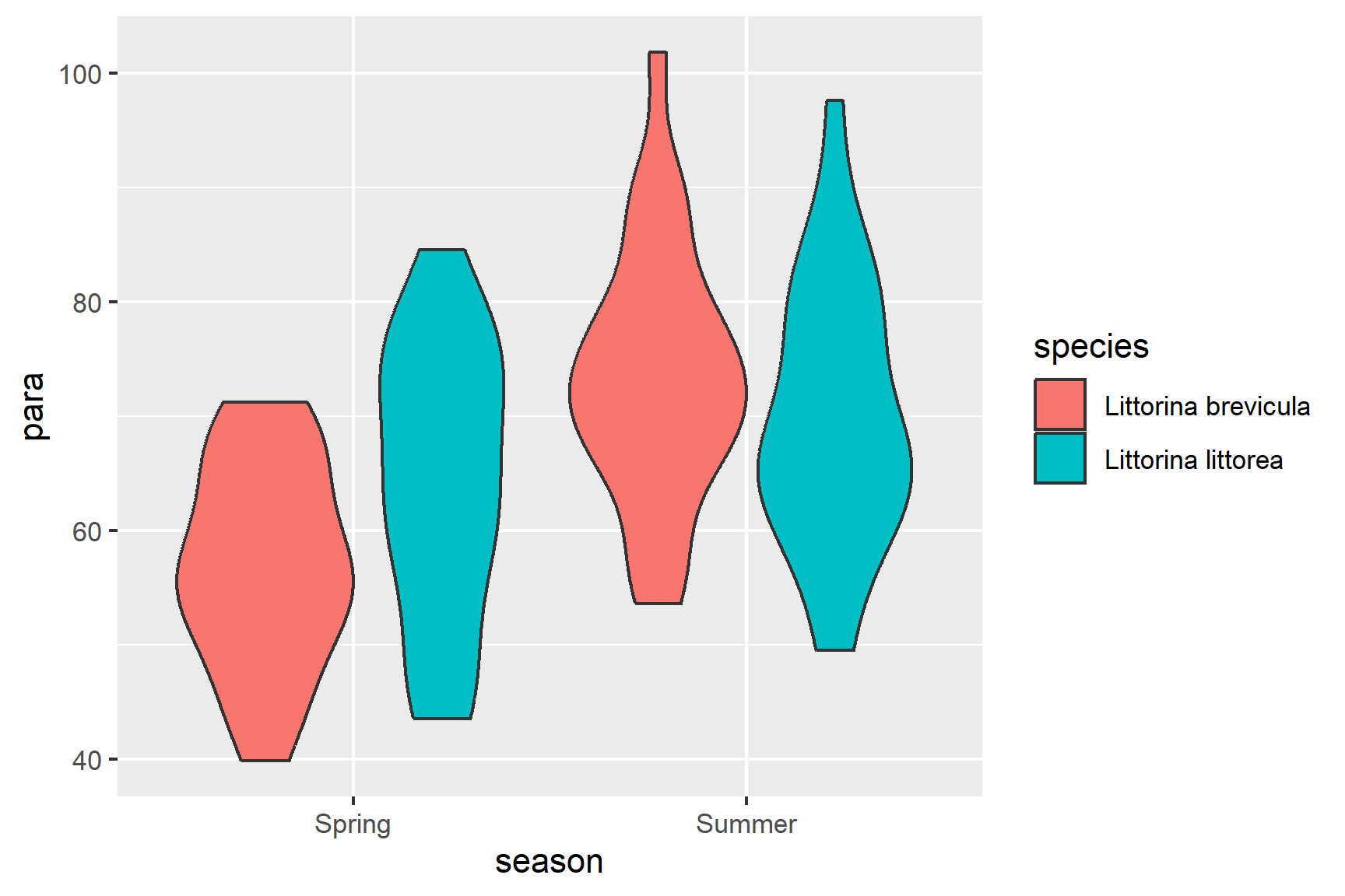

Figure 15.2: The parasite load for two species of Littorina indicated by the fill colour, in the Spring and Summer. Parasite load seems to be higher for both species in the summer and that effect looks bigger in L.brevicula - it has the lowest spring mean but the highest summer mean.

R will order the groups alphabetically by default.

The figure suggests that parasite load is higher for both species in the summer and that effect looks bigger in L.brevicula - it has the lowest spring mean but the highest summer mean.

Summarising the data for each species-season combination is the next sensible step. The most useful summary statistics are the means, standard deviations, sample sizes and standard errors. I recommend the group_by() and summarise() approach:

peri_summary <- periwinkle |>  
  group_by(season, species) |>  
  summarise(mean = mean(para),
            sd = sd(para),
            n = length(para),
            se = sd / sqrt(n))

We have save the results to peri_summary so that we can use the means and standard errors in our plot later.

peri_summary
## # A tibble: 4 × 6
## # Groups:   season [2]
##   season species              mean    sd     n    se
##   <chr>  <chr>               <dbl> <dbl> <int> <dbl>
## 1 Spring Littorina brevicula  57.0  8.83    25  1.77
## 2 Spring Littorina littorea   64.2 11.9     25  2.38
## 3 Summer Littorina brevicula  73.5 11.2     25  2.24
## 4 Summer Littorina littorea   69.9 11.5     25  2.30

The summary confirms both species have a higher mean in the summer and that the difference between the species is reversed - L.brevicula minus L.littorea is -7.2588 in the spring but 3.6328 in summer.

15.3.2 Apply lm()

We can create a two-way ANOVA model like this:

mod <- lm(data = periwinkle, para ~ species * season)

And examine the model with:

summary(mod)
## 
## Call:
## lm(formula = para ~ species * season, data = periwinkle)
## 
## Residuals:
##     Min      1Q  Median      3Q     Max 
## -20.711  -6.308  -1.120   8.085  28.269 
## 
## Coefficients:
##                                        Estimate Std. Error t value Pr(>|t|)    
## (Intercept)                              56.972      2.185  26.073  < 2e-16 ***
## speciesLittorina littorea                 7.259      3.090   2.349   0.0209 *  
## seasonSummer                             16.568      3.090   5.362 5.68e-07 ***
## speciesLittorina littorea:seasonSummer  -10.892      4.370  -2.492   0.0144 *  
## ---
## Signif. codes:  0 '***' 0.001 '**' 0.01 '*' 0.05 '.' 0.1 ' ' 1
## 
## Residual standard error: 10.93 on 96 degrees of freedom
## Multiple R-squared:  0.2547, Adjusted R-squared:  0.2314 
## F-statistic: 10.94 on 3 and 96 DF,  p-value: 3.043e-06

The Estimates in the Coefficients table give:

• (Intercept) known as \(\beta_0\). This the mean of the group with the first level of both explanatory variables, i.e., the mean of L.brevicula group in Spring. Just as the intercept is the value of y (the response) when the value of x (the explanatory) is zero in a simple linear regression, this is the value of para when both season and species are at their first levels. The order of the levels is alphabetical by default.

• speciesLittorina littorea known as \(\beta_1\). This is what needs to be added to the L.brevicula Spring mean (the intercept) when the species goes from its first level to its second. That is, it is the difference between the L.brevicula and L.littorea means in Spring. The speciesLittorina littorea estimate is positive so the the L.littorea mean is higher than the L.brevicula mean in Spring. If we had more species we would have more estimates beginning species... and all would be comparisons to the intercept.

• seasonSummer known as \(\beta_2\). This is what needs to be added to the L.brevicula Spring mean (the intercept) when the season goes from its first level to its second. That is, it is the difference between the Spring and Summer means for L.brevicula. The seasonSummer estimate is positive so the the Summer mean is higher than the Spring mean. If we had more seasons we would have more estimates beginning season... and all would be comparisons to the intercept.

• speciesLittorina littorea:seasonSummer known as \(\beta_3\). This is interaction effect. It is an additional effect. Going from L.brevicula to L.littorea adds \(\beta_1\) to the intercept. Going from Spring to Summer adds \(\beta_2\) to the intercept. Going from L.brevicula in Spring to L.littorea in Summer adds \(\beta_1 + \beta_2 + \beta_3\) to the intercept. If \(\beta_3\) is zero then the effect of species is the same in both seasons. If \(\beta_3\) is not zero then the effect of species is different in the two seasons.

The p-values on each line are tests of whether that coefficient is different from zero.

The F value and p-value in the last line are a test of whether the model as a whole explains a significant amount of variation in the response variable. The model of season and species overall explains a significant amount of the variation in parasite load (p-value: 3.043e-06). To see which of the three effects are significant we can use the anova() function on our model.

Determine which effects are significant:

anova(mod)
## Analysis of Variance Table
## 
## Response: para
##                Df  Sum Sq Mean Sq F value    Pr(>F)    
## species         1    82.2   82.17  0.6884   0.40876    
## season          1  3092.8 3092.81 25.9108 1.778e-06 ***
## species:season  1   741.4  741.42  6.2114   0.01441 *  
## Residuals      96 11458.9  119.36                      
## ---
## Signif. codes:  0 '***' 0.001 '**' 0.01 '*' 0.05 '.' 0.1 ' ' 1

The parasite load is significantly greater in Summer (F = 25.9; d.f. = 1, 96; p < 0.0001) but this effect differs between species (F = 6.2; d.f. = 1,96; p = 0.014) with a greater increase in parasite load in L.brevicula than in L.littorea.

We need a post-hoc test to see which comparisons are significant and can again use then emmeans (Lenth 2023) package.

Load the package

library(emmeans)

Carry out the post-hoc test

emmeans(mod, ~ species * season) |> pairs()
##  contrast                                                estimate   SE df
##  Littorina brevicula Spring - Littorina littorea Spring     -7.26 3.09 96
##  Littorina brevicula Spring - Littorina brevicula Summer   -16.57 3.09 96
##  Littorina brevicula Spring - Littorina littorea Summer    -12.94 3.09 96
##  Littorina littorea Spring - Littorina brevicula Summer     -9.31 3.09 96
##  Littorina littorea Spring - Littorina littorea Summer      -5.68 3.09 96
##  Littorina brevicula Summer - Littorina littorea Summer      3.63 3.09 96
##  t.ratio p.value
##   -2.349  0.0943
##   -5.362  <.0001
##   -4.186  0.0004
##   -3.013  0.0172
##   -1.837  0.2625
##    1.176  0.6436
## 
## P value adjustment: tukey method for comparing a family of 4 estimates

Each row is a comparison between the two means in the ‘contrast’ column. The ‘estimate’ column is the difference between those means and the ‘p.value’ indicates whether that difference is significant.

A plot can be used to visualise the result of the post hoc which can be especially useful when there are very many comparisons.

Plot the results of the post-hoc test:

emmeans(mod, ~ species * season) |> plot()

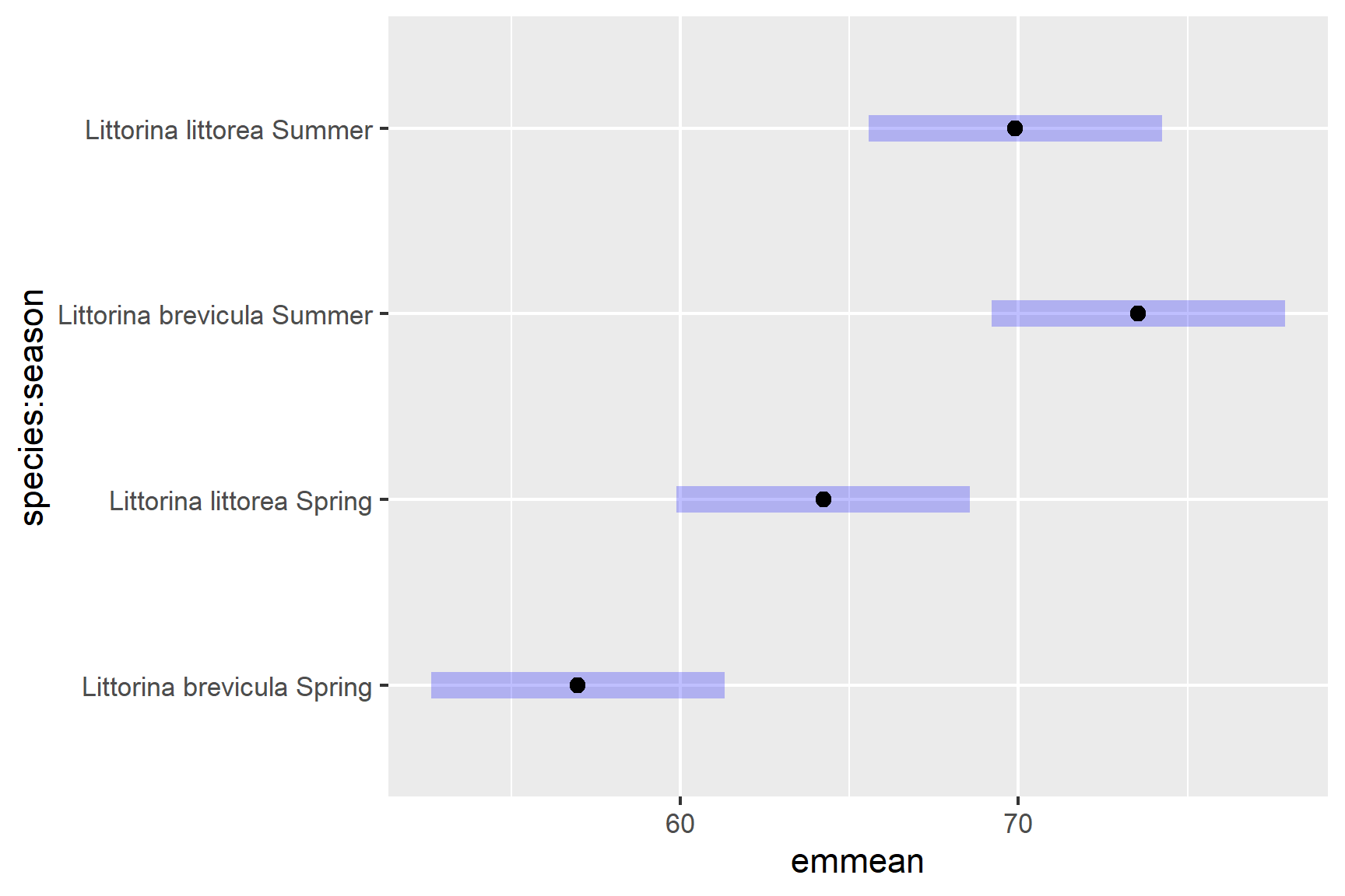
We have significant differences between:

• L.brevicula in the Spring and Summer p <.0001
• L.brevicula in the Spring and L.littorea in the Summer p = 0.0004
• L.littorea in the Spring L.brevicula in the Summer p = 0.0172

15.3.3 Check assumptions

Check the assumptions: All general linear models assume the “residuals” are normally distributed and have “homogeneity” of variance.

Our first check of these assumptions is to use common sense: diameter is a continuous and we would expect it to be normally distributed thus we would expect the residuals to be normally distributed thus we would expect the residuals to be normally distributed

We then proceed by plotting residuals. The plot() function can be used to plot the residuals against the fitted values (See Figure 15.3). This is a good way to check for homogeneity of variance.

plot(mod, which = 1)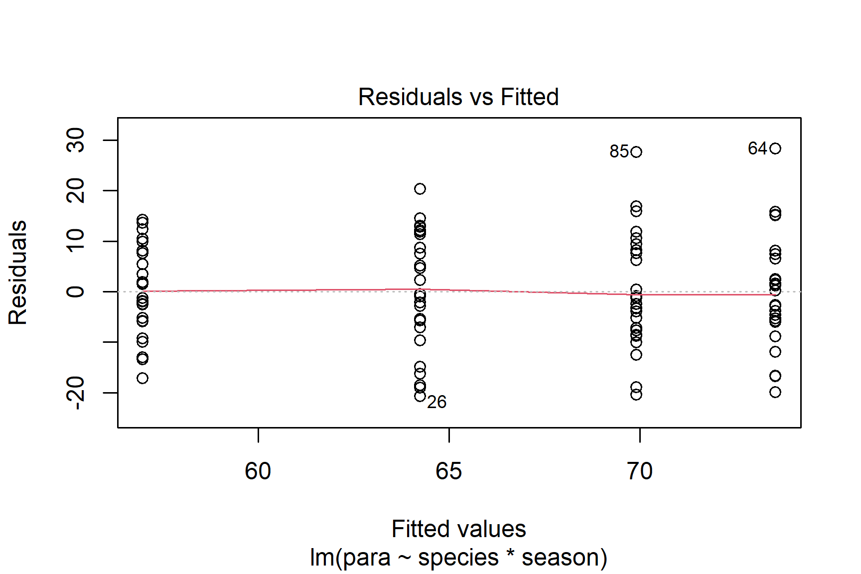

Figure 15.3: A plot of the residuals against the fitted values shows whether the points are distributed similarly in each group. Any difference seems small but perhaps the residuals are less variable for the lowest mean.

We can also use a histogram to check for normality (See Figure 15.4).

ggplot(mapping = aes(x = mod$residuals)) + 
  geom_histogram(bins = 10)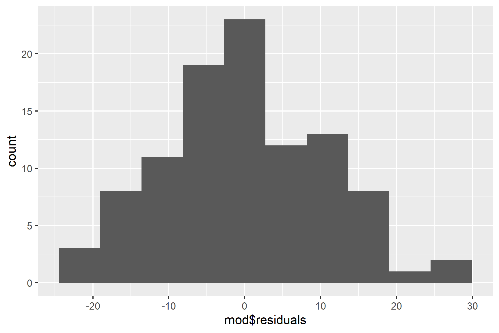

Figure 15.4: A histogram of residuals is symetrical and seems consistent with a normal distribution. This is a good sign for the assumption of normally distributed residuals.

Finally, we can use the Shapiro-Wilk test to test for normality.

shapiro.test(mod$residuals)
## 
##  Shapiro-Wilk normality test
## 
## data:  mod$residuals
## W = 0.98424, p-value = 0.2798

The p-value is greater than 0.05 so this test of the normality assumption is not significant.

Taken together, these results suggest that the assumptions of normality and homogeneity of variance are probably not violated.

15.3.4 Report

We might report this result as:

The parasite load was significantly greater in Summer (F = 25.9; d.f. = 1, 96; p < 0.0001) but this effect differed between species (F = 6.2; d.f. = 1,96; p = 0.014) with a greater increase in parasite load in L.brevicula (from \(\bar{x} \pm s.e\): 57.0 \(\pm\) 1.77 units to 73.5 \(\pm\) 2.24 units) than in L.littorea (from 64.2 \(\pm\) 2.38 units to 69.9 \(\pm\) 2.30 units). See Figure 15.5.

ggplot() +
  geom_point(data = periwinkle, aes(x = season,
                                    y = para,
                                    shape = species),
             position = position_jitterdodge(dodge.width = 1,
                                             jitter.width = 0.4,
                                             jitter.height = 0),
             size = 3,
             colour = "gray50") +
  geom_errorbar(data = peri_summary, 
                aes(x = season, ymin = mean - se, ymax = mean + se, group = species),
                linewidth = 0.4, size = 1,
                position = position_dodge(width = 1)) +
  geom_errorbar(data = peri_summary, 
                aes(x = season, ymin = mean, ymax = mean, group = species),
                linewidth = 0.3, size = 1,
                position = position_dodge(width = 1) ) +
  scale_x_discrete(name = "Season") +
  scale_y_continuous(name = "Number of parasites",
                     expand = c(0, 0),
                     limits = c(0, 140)) +
  scale_shape_manual(values = c(19, 1),
                     name = NULL,
                     labels = c(bquote(italic("L.brevicula")),
                                bquote(italic("L.littorea")))) +
  # *L.brevicula* in the Spring and Summer `p <0.0001`
  annotate("segment",
           x = 0.75, xend = 1.75,
           y = 115, yend = 115,
           colour = "black") +
  annotate("text",
           x = 1.25,  y = 119,
           label = "p < 0.0001") +
  # # *L.brevicula* in the Spring and  *L.littorea* in the Summer `p = 0.0004`
  annotate("segment",
           x = 0.75, xend = 2.25,
           y = 125, yend = 125,
           colour = "black") +
  annotate("text", x = 1.5,  y = 129,
           label = "p = 0.0004") +
  # *L.littorea* in the Spring *L.brevicula* in the Summer `p = 0.0172`
  annotate("segment",
           x = 1.25, xend = 1.75,
           y = 105, yend = 105,
           colour = "black") +
  annotate("text", x = 1.5,  y = 109,
           label = "p = 0.0172") +
  theme_classic() +
  theme(legend.title = element_blank(),
        legend.position = c(0.85, 0.15)) 

Figure 15.5: Parasite load is greater in Summer especially for L.brevicula. Live specimens of two species of periwinkle, L.brevicula and L.littorea were collected from sites in northern England in the Spring and Summer and gut parasite load was determined. Error bars are means \(\pm\) 1 standard error. Parasite load was significantly greater in Summer (F = 25.9; d.f. = 1, 96; p < 0.0001) but this effect differed between species (F = 6.2; d.f. = 1,96; p = 0.014) with a greater increase in parasite load in L.brevicula than in L.littorea. Data analysis was conducted in R (R Core Team 2023) with tidyverse packages (Wickham et al. 2019). Post-hoc analysis was carried out with Tukey’s Honestly Significant Difference test (Tukey 1949).

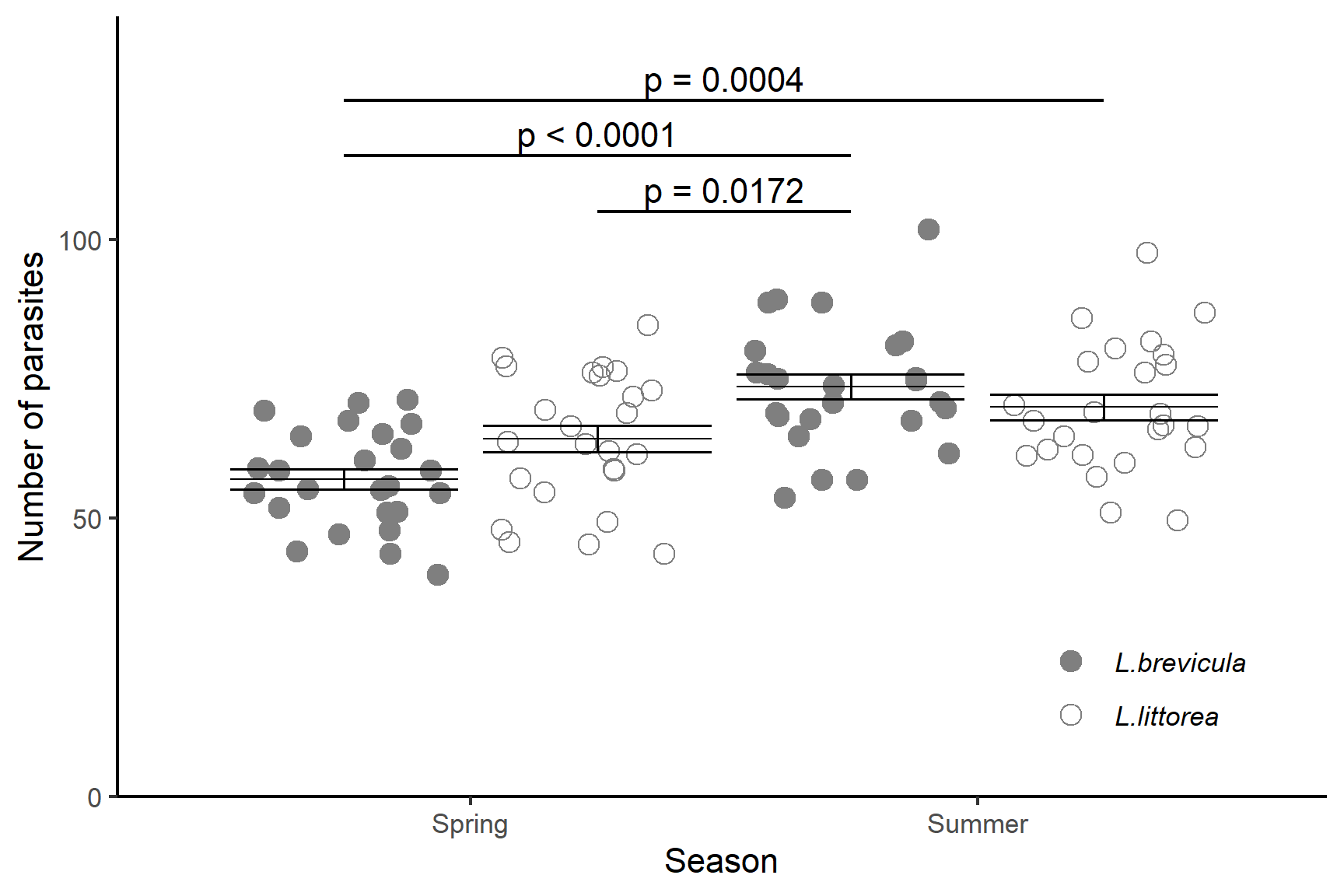
15.4 Summary

1. A linear model with two explanatory variable with two or more groups each is also known as a two-way ANOVA.

2. We estimate the coefficients (also called the parameters) of the model. For a two-way ANOVA with two groups in each explanatory variable these are

   • the mean of the group with the first level of both explanatory variables \(\beta_0\),
   • what needs to be added to \(\beta_0\) when one of the explanatory variables goes from its first level to its second, \(\beta_1\)
   • what needs to be added to \(\beta_0\) when the other of the explanatory variables goes from its first level to its second, \(\beta_2\)
   • \(\beta_3\), the interaction effect: what additionally needs to be added to \(\beta_0\) + \(\beta_1\) + \(\beta_2\) when both of the explanatory variables go from their first level to their second

3. We can use lm() to two-way ANOVA in R.

4. In the output of lm() the coefficients are listed in a table in the Estimates column. The p-value for each coefficient is in the test of whether it differs from zero. At the bottom of the output there is an \(F\) test of the model overall. The R-squared value is the proportion of the variance in the response variable that is explained by the model.

5. To see which of the three effects are significant we can use the anova() function on our model.

6. To find out which means differ, we need a post-hoc test. Here we use Tukey’s HSD applied with the emmeans() and pairs() functions from the emmeans package. Post-hoc tests make adjustments to the p-values to account for the fact that we are doing multiple tests.

7. The assumptions of the general linear model are that the residuals are normally distributed and have homogeneity of variance. A residual is the difference between the predicted value and the observed value.

8. We examine a histogram of the residuals and use the Shapiro-Wilk normality test to check the normality assumption. We check the variance of the residuals is the same for all fitted values with a residuals vs fitted plot.

9. When reporting the results of a test we give the significance, direction and size of the effect. We use means and standard errors for parametric tests like two-way ANOVA. We also give the test statistic, the degrees of freedom (parametric) or sample size (non-parametric) and the p-value. We annotate our figures with the p-value, making clear which comparison it applies to.

Lenth, Russell V. 2023. “Emmeans: Estimated Marginal Means, Aka Least-Squares Means.” https://CRAN.R-project.org/package=emmeans.

R Core Team. 2023. R: A Language and Environment for Statistical Computing. Vienna, Austria: R Foundation for Statistical Computing. https://www.R-project.org/.

Tukey, John W. 1949. “Comparing Individual Means in the Analysis of Variance.” Biometrics 5 (2): 99–114. https://doi.org/10.2307/3001913.

Wickham, Hadley. 2014. “Tidy Data.” Journal of Statistical Software, Articles 59 (10): 1–23. https://vita.had.co.nz/papers/tidy-data.pdf.

Wickham, Hadley, Mara Averick, Jennifer Bryan, Winston Chang, Lucy D’Agostino McGowan, Romain François, Garrett Grolemund, et al. 2019. “Welcome to the Tidyverse” 4: 1686. https://doi.org/10.21105/joss.01686.