13  Two-Sample tests

Just needs proof reading

You are reading a work in progress. This page is compete but needs final proof reading.

13.1 Overview

In the last chapter we learned about single linear regression, a technique used when the explanatory variable is continuous. We now turn our attention to cases where our explanatory variable is categorical and has two groups. For example, we might want to know if there is a difference in mass between two subspecies of chaffinch, or if marks in two subjects are the same.

We use lm() or wilcox.test() to carry out a two-sample test depending on whether the assumptions of lm() are met. The general linear models applied with lm() are based on the normal distribution and known as parametric tests because they use the parameters of the normal distribution (the mean and standard deviation) to determine if an effect is significant. Null hypotheses are about a mean or difference between means. The assumptions need to be met for the p-values generated to be accurate.

If the assumptions are not met, we can use alternatives known as non-parametric tests. Non-parametric tests are based on the ranks of values rather than the actual values themselves. Null hypotheses are about the mean rank rather than the mean. These tests have fewer assumptions and can be used in more situations but the downside is they tend to be less powerful. This means they are less able to detect a difference where one exists.

13.1.1 Independent samples and paired samples.

An important consideration in conducting tests is whether the values in one group are independent of the values in another group. Non-independence occurs when the two measures are linked in some way. The link could be that they are from the same individual, the same time or the same location. For example, if we want to evaluate a treatment for high blood pressure we might measure blood pressure before and after the treatment on the same individuals. This would mean the before and after measures were not independent. If pairs of observations in different groups have something in common that make them more similar to each other than to other observations, then those observations are not independent. We use a different testing approach for independent and non-independent samples.

13.1.2 T-tests

A linear model with one explanatory variable with two groups is also known as a two-sample t-test when the samples are independent and as a paired-samples t-test when they are not. R does have a t.test() function which allows you to fit a linear model with just two groups. However, here we teach you to use and interpret the lm() function because it is more generalisable. You can use lm() when you have three or more groups or additional explanatory variables. The output of lm() is also in the same form as many other statistical functions in R. This means what you learn in performing t-tests with lm() will help you learn other methods more easily. However, it is definitely not wrong to use t.test() rather than lm() for two-group situations - the procedures are identical and the p-values will be the same.

13.1.3 Model assumptions

The assumptions of the general linear model are that the residuals are normally distributed and have homogeneity of variance. A residual is the difference between the predicted value and the observed value.

If we have a continuous response and a categorical explanatory variable with two groups, we usually apply the general linear model with lm() and then check the assumptions, however, we can sometimes tell when a non-parametric test would be more appropriate before that:

• Use common sense - the response should be continuous (or nearly continuous, see Ideas about data: Theory and practice). Consider whether you would expect the response to be continuous.

• We expect decimal places and few repeated values.

To examine the assumptions after fitting the linear model, we plot the residuals and test them against the normal distribution in the same way as we did for single linear regression.

13.1.4 Reporting

In reporting the result of two-sample test we give:

1. the significance of effect - whether there is there a difference between the groups

   • parametric: whether there is there a difference between the groups means
   • non-parametric: whether there is there a difference between the group medians

2. the direction of effect - which of the means/medians is greater

3. the magnitude of effect - how big is the difference between the means/medians

   • parametric: the means and standard errors for each group or the mean difference for paired samples
   • non-parametric: the medians for each group or the median difference for paired samples

Figures should reflect what you have said in the statements. Ideally they should show both the raw data and the statistical model:

• parametric: means and standard errors
• non-parametric: boxplots with medians and interquartile range

We will explore all of these ideas with some examples.

13.2 🎬 Your turn!

If you want to code along you will need to start a new RStudio project, add a data-raw folder and open a new script. You will also need to load the tidyverse package (Wickham et al. 2019).

13.3 Two independent samples, parametric

A number of subspecies of the common chaffinch, Fringilla coelebs, have been described based principally on the differences in the pattern and colour of the adult male plumage (Suárez et al. 2009). Two of groups of these subspecies are:

• the “coelebs group” (Figure 13.1 (a)) that occurs in Europe and Asia
• the “canariensis group” (Figure 13.1 (b)) that occurs on the Canary Islands.

(a) F. c. coelebs

(b) F. c. palmae

Figure 13.1: Adult male Fringilla coelebs of the coelebs group on the left (Andreas Trepte, CC BY-SA 2.5 https://creativecommons.org/licenses/by-sa/2.5, via Wikimedia Commons) and of the canariensis group on the right (H. Zell, CC BY-SA 3.0 https://creativecommons.org/licenses/by-sa/3.0, via Wikimedia Commons).

The data in chaff.txt give the masses of twenty individuals from each subspecies. We want to know if the subspecies differ in mass. These groups are independent - there is no link between values in one group and any value in the other group. In this scenario our null hypothesis, \(H_0\), is that there is no difference between the two subspecies in mass or that subspecies has no effect on mass. This is written as: \(H_0: \beta_1 = 0\).

13.3.1 Import and explore

Import the data:

chaff <- read_table("data-raw/chaff.txt")

subspecies	mass
coelebs	18.3
coelebs	22.1
coelebs	22.4
coelebs	18.5
coelebs	22.2
coelebs	19.3
coelebs	17.8
coelebs	20.2
coelebs	22.1
coelebs	16.6
coelebs	20.7
coelebs	18.7
coelebs	22.6
coelebs	21.5
coelebs	21.7
coelebs	19.9
coelebs	23.1
coelebs	17.8
coelebs	19.5
coelebs	24.6
canariensis	22.7
canariensis	20.6
canariensis	25.4
canariensis	20.4
canariensis	21.6
canariensis	17.0
canariensis	26.4
canariensis	20.4
canariensis	24.7
canariensis	21.8
canariensis	23.4
canariensis	24.4
canariensis	21.0
canariensis	23.4
canariensis	20.5
canariensis	21.4
canariensis	21.5
canariensis	23.7
canariensis	23.4
canariensis	21.8

These data are in tidy format (Wickham 2014) - all the mass values are in one column with another column indicating the subspecies. This means they are well formatted for analysis and plotting.

In the first instance, it is always sensible to create a rough plot of our data. This is to give us an overview and help identify if there are any issues like missing or extreme values. It also gives us idea what we are expecting from the analysis which will make it easier for us to identify if we make some mistake in applying that analysis.

Violin plots (geom_violin()), box plots (geom_boxplot(), see Figure 13.2) or scatter plots (geom_point()) all make good choices for exploratory plotting and it does not matter which of these you choose.

ggplot(data = chaff,
       aes(x = subspecies, y = mass)) +
  geom_boxplot()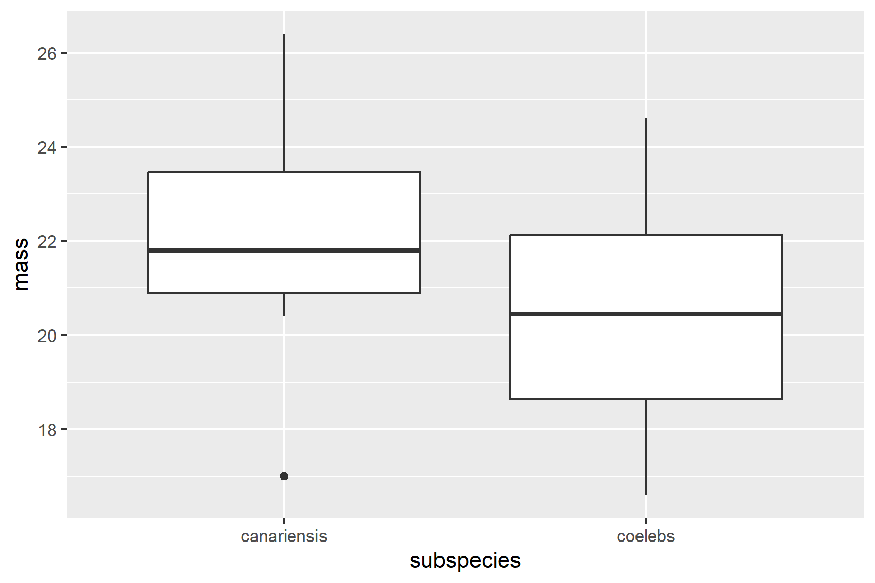

Figure 13.2: The mass of two subspecies of chaffinch. A boxplot is a useful way to get an overview of the data and helps us identify any issues such as missing or extreme values. It also tells us what to expect from the analysis.

R will order the groups alphabetically by default.

The figure suggests that the canariensis group is heavier than the coelebs group.

Summarising the data for each subspecies group is the next sensible step. The most useful summary statistics are the means, standard deviations, sample sizes and standard errors. I recommend the group_by() and summarise() approach:

chaff_summary <- chaff |> 
  group_by(subspecies) |> 
  summarise(mean = mean(mass),
            std = sd(mass),
            n = length(mass),
            se = std/sqrt(n))

We have save the results to chaff_summary so that we can use the means and standard errors in our plot later.

chaff_summary
## # A tibble: 2 × 5
##   subspecies   mean   std     n    se
##   <chr>       <dbl> <dbl> <int> <dbl>
## 1 canariensis  22.3  2.15    20 0.481
## 2 coelebs      20.5  2.14    20 0.478

13.3.2 Apply lm()

We can create a two-sample model like this:

mod <- lm(data = chaff, mass ~ subspecies)

And examine the model with:

summary(mod)
## 
## Call:
## lm(formula = mass ~ subspecies, data = chaff)
## 
## Residuals:
##     Min      1Q  Median      3Q     Max 
## -5.2750 -1.7000 -0.3775  1.6200  4.1250 
## 
## Coefficients:
##                   Estimate Std. Error t value Pr(>|t|)    
## (Intercept)        22.2750     0.4795  46.456   <2e-16 ***
## subspeciescoelebs  -1.7950     0.6781  -2.647   0.0118 *  
## ---
## Signif. codes:  0 '***' 0.001 '**' 0.01 '*' 0.05 '.' 0.1 ' ' 1
## 
## Residual standard error: 2.144 on 38 degrees of freedom
## Multiple R-squared:  0.1557, Adjusted R-squared:  0.1335 
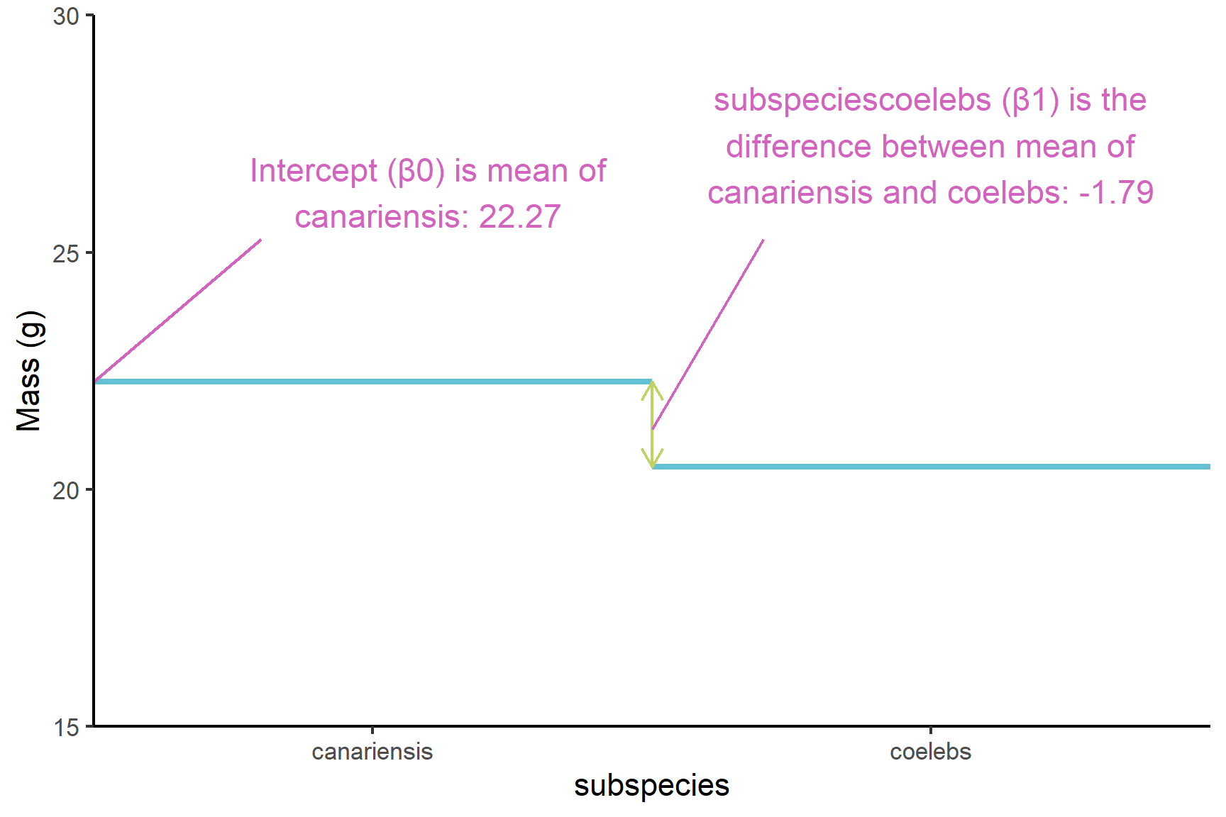
## F-statistic: 7.007 on 1 and 38 DF,  p-value: 0.01175

The Estimates in the Coefficients table give:

• (Intercept) known as \(\beta_0\). The mean of the canariensis group (Figure 13.3). Just as the intercept is the value of the y (the response) when the value of x (the explanatory) is zero in a simple linear regression, this is the value of mass when the subspecies is at its first level. The order of the levels is alphabetical by default.

• subspeciescoelebs, known as \(\beta_1\), is what needs to be added to the mean of the canariensis group to get the mean of the coelebs group (Figure 13.3). Just as the slope is amount of y that needs to be added for each unit of x in a simple linear regression, this is the amount of mass that needs to be added when the subspecies goes from its first level to its second level (i.e., one unit). The subspeciescoelebs estimate is negative so the the coelebs group mean is lower than the canariensis group mean

The p-values on each line are tests of whether that coefficient is different from zero. Thus it is:

subspeciescoelebs -1.7950 0.6781 -2.647 0.0118 *

that tells us the difference between the means is significant.

The F value and p-value in the last line are a test of whether the model as a whole explains a significant amount of variation in the response variable. For a two-sample test, just like a regression, this is exactly equivalent to the test of the slope against zero and the two p-values will be the same.

Figure 13.3: In a two-sample linear model, the first estimate is the intercept which is the mean of the first group. The second estimate is the ‘slope’ which is what has to added to the intercept to get the second group mean. Note that y axis starts at 15 to create more space for the annotations.

13.3.3 Check assumptions

Check the assumptions: All general linear models assume the “residuals” are normally distributed and have “homogeneity” of variance.

Our first check of these assumptions is to use common sense: mass is a continuous variable and we would expect it to be normally distributed thus we would also expect the residuals to be normally distributed.

We then plot the residuals. The plot() function can be used to plot the residuals against the fitted values (See Figure 13.4). This is a good way to check for homogeneity of variance.

plot(mod, which = 1)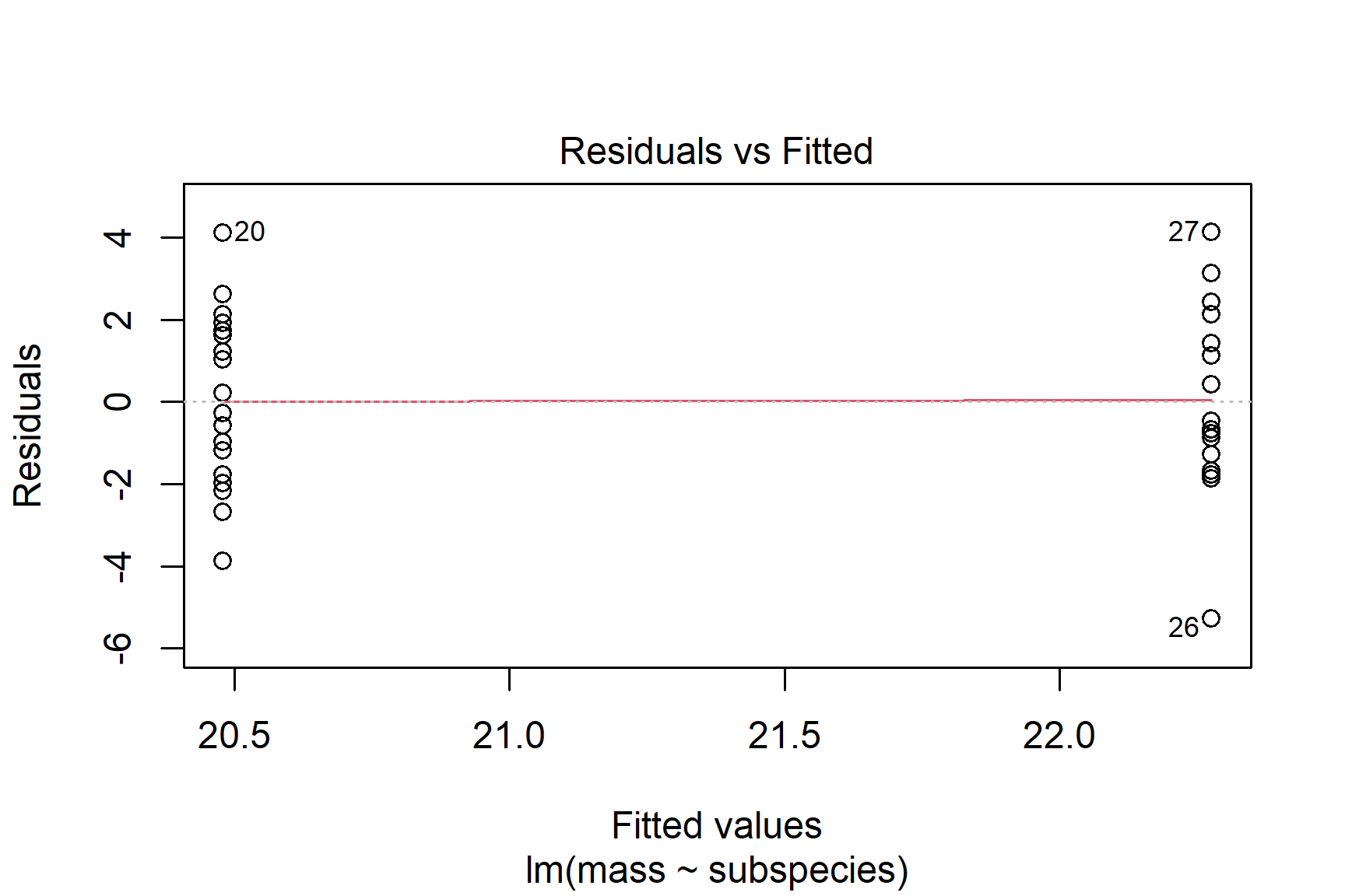

Figure 13.4: A plot of the residuals against the fitted values shows the points are distributed similarly in each group. This is a good sign for the assumption of homogeneity of variance.

We can also use a histogram to check for normality (See Figure 13.5).

ggplot(mapping = aes(x = mod$residuals)) + 
  geom_histogram(bins = 10)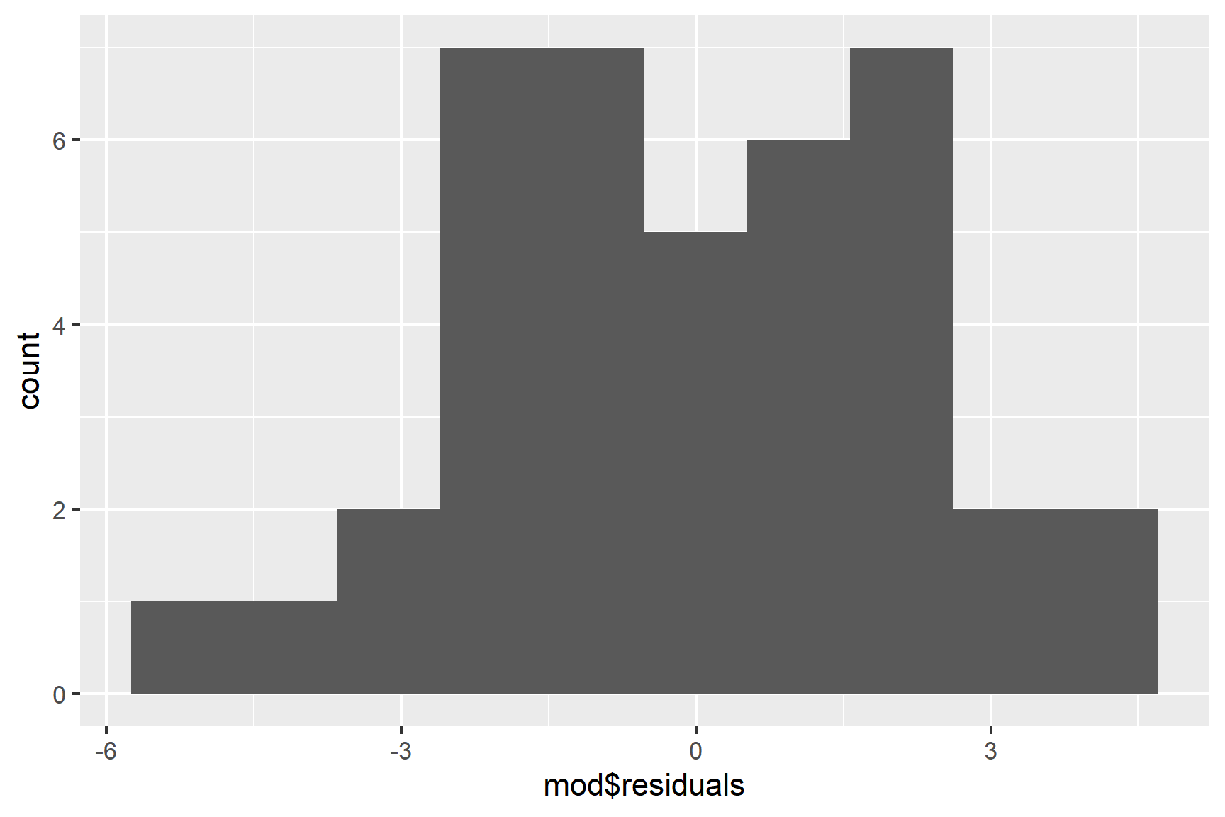

Figure 13.5: A histogram of residuals is symetrical and seems consistent with a normal distribution. This is a good sign for the assumption of normally distributed residuals.

Finally, we can use the Shapiro-Wilk test to test for normality.

shapiro.test(mod$residuals)
## 
##  Shapiro-Wilk normality test
## 
## data:  mod$residuals
## W = 0.98046, p-value = 0.7067

The p-value is greater than 0.05 so this test of the normality assumption is not significant.

Taken together, these results suggest that the assumptions of normality and homogeneity of variance are not violated.

13.3.4 Report

Canariensis chaffinches (\(\bar{x} \pm s.e\): 22.48 \(\pm\) 0.48) were significantly heavier than Coelebs (20.28 \(\pm\) 0.48 ) (t = 2.65; d.f. = 38; p = 0.012). See Figure 13.6.

ggplot() +
  geom_point(data = chaff, aes(x = subspecies, y = mass),
             position = position_jitter(width = 0.1, height = 0),
             colour = "gray50") +
  geom_errorbar(data = chaff_summary, 
                aes(x = subspecies, ymin = mean - se, ymax = mean + se),
                width = 0.3) +
  geom_errorbar(data = chaff_summary, 
                aes(x = subspecies, ymin = mean, ymax = mean),
                width = 0.2) +
  scale_y_continuous(name = "Mass (g)", 
                     limits = c(0, 30), 
                     expand = c(0, 0)) +
  scale_x_discrete(name = "Subspecies", 
                   labels = c("Canariensis", "Coelebs")) +
  annotate("segment", x = 1, xend = 2, 
           y = 28, yend = 28,
           colour = "black") +
  annotate("text", x = 1.5,  y = 29, 
           label = expression(italic(p)~"= 0.012")) +
  theme_classic()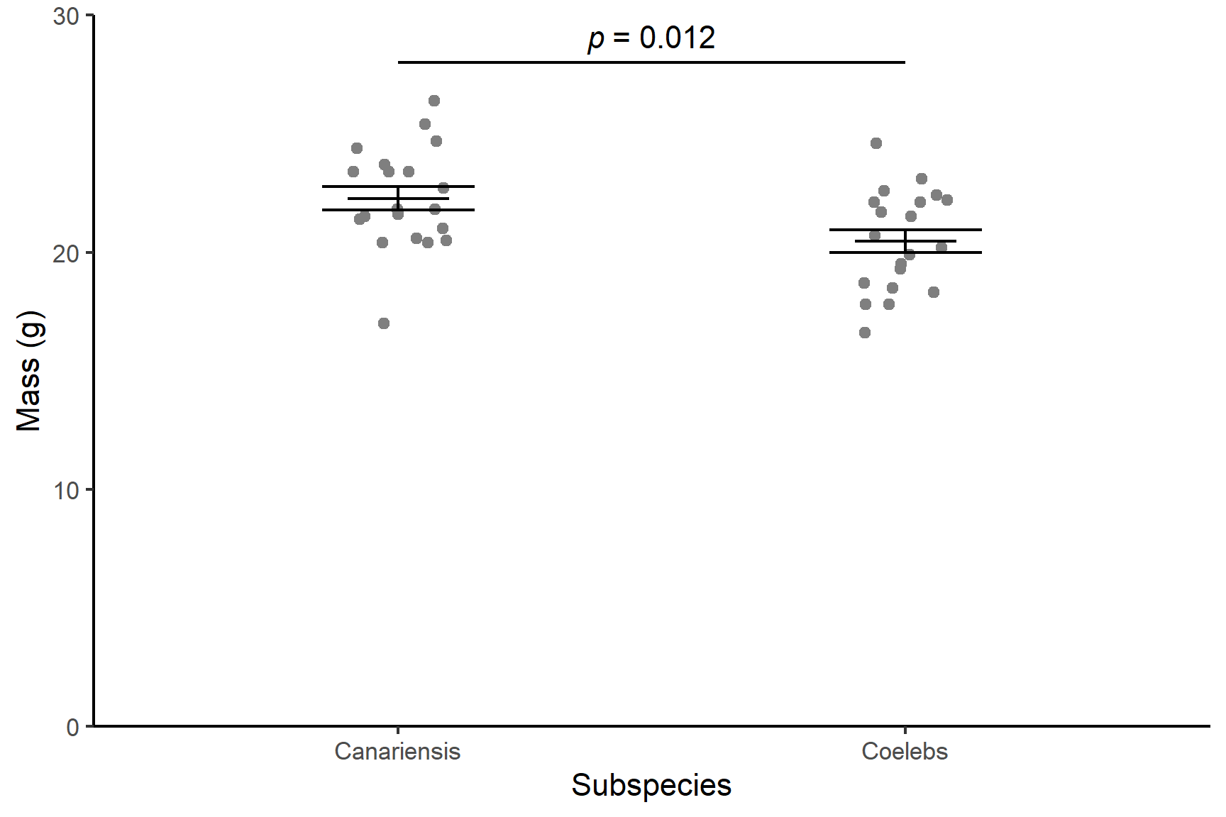

Figure 13.6: Canariensis chaffinches are heavier than Coelebs chaffinches. The mean mass of 20 randomly sampled males from each subspecies was determined. Error bars are \(\pm\) 1 standard error. Canariensis chaffinches were significantly heavier than Coelebs (t = 2.65; d.f. = 38; p = 0.012). Data analysis was conducted in R (R Core Team 2024) with tidyverse packages (Wickham et al. 2019).

13.4 Two independent samples, non-parametric

The non-parametric equivalent of the linear model with two independent samples is the “Wilcoxon rank sum test” (Wilcoxon 1945). It is commonly also known as the Mann-Whitney or Wilcoxon–Mann–Whitney.

The general question you have about your data - are these two groups different - is the same, but one of more of the following is true:

• the response variable is not continuous
• the residuals are not normally distributed
• the sample size is too small to tell if they are normally distributed.
• the variance is not homogeneous

The test is a applied in R with the wilcox.test() function.

The data in arabidopsis.txt give the number of leaves on eight wildtype and eight mutant Arabidopsis thaliana plants. We want to know if the two types of plants have differing numbers of leaves. These are counts, so they are not continuous and the sample sizes are quite small. A non-parametric test is a safer option. In this scenario our null hypothesis, \(H_0\), is that there is no difference between the two types of plant in the number of leaves.

13.4.1 Import and explore

arabidopsis <- read_table("data-raw/arabidopsis.txt")

These data are in tidy format (Wickham 2014) - the numbers of leaves are in one column with another column indicating whether the observation comes from a wildtype or mutant Arabidopsis. This means they are well formatted for analysis and plotting.

Create a quick plot of the data:

ggplot(data = arabidopsis, 
       aes(x = type, y = leaves)) +
  geom_boxplot()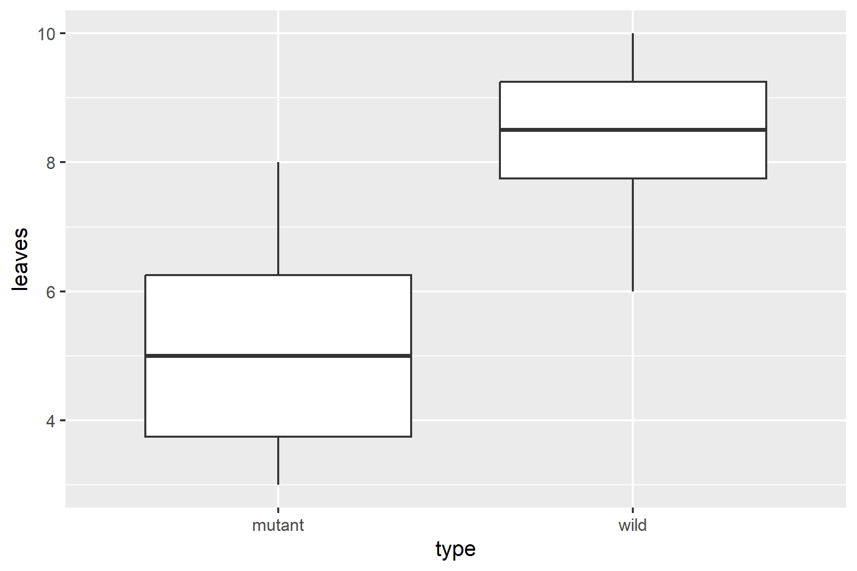

Figure 13.7: The number of leaves on mutant and wildtype plants. A boxplot is a useful way to get an overview of the data and helps us identify any issues such as missing or extreme values. It also tells us what to expect from the analysis.

Our rough plot shows that the mutant plants have fewer leaves than the wildtype plants.

Summarising the data using the median and interquartile range is more aligned to the type of data and the type of analysis than using means and standard deviations:

arabidopsis_summary <- arabidopsis |> 
  group_by(type) |> 
  summarise(median = median(leaves),
            interquartile  = IQR(leaves),
            n = length(leaves))

View the results:

arabidopsis_summary
## # A tibble: 2 × 4
##   type   median interquartile     n
##   <chr>   <dbl>         <dbl> <int>
## 1 mutant    5             2.5     8
## 2 wild      8.5           1.5     8

13.4.2 Apply wilcox.test()

We pass the dataframe and variables to wilcox.test() in the same way as we did for lm(). We give the data argument and a “formula” which says leaves ~ type meaning “explain leaves by type”.

wilcox.test(data = arabidopsis, leaves ~ type)
## 
##  Wilcoxon rank sum test with continuity correction
## 
## data:  leaves by type
## W = 5, p-value = 0.005051
## alternative hypothesis: true location shift is not equal to 0

The warning message “Warning: cannot compute exact p-value with ties” is not something to worry about too much. It is a warning rather than an indication that your results are incorrect. It means the p -value is based on an approximation rather than being exact because there are ties (some values are the same).

The result of the test is given on this line: W = 5, p-value = 0.005051. W is the test statistic. The p-value is less than 0.05 meaning there is a significant difference in the number of leaves on wildtype and mutant plants.

13.4.3 Report

There are significantly more leaves on wildtype (median = 8.5) than mutant (median = 5) plants (Wilcoxon rank sum test: W = 5, \(n_1\) = 8, \(n_2\) = 8, p = 0.005). See Figure 13.8.

ggplot(data = arabidopsis, 
       aes(x = type, y = leaves)) +
  geom_boxplot() +
  scale_y_continuous(name = "Number of leaves", 
                     limits = c(0, 12), 
                     expand = c(0, 0)) +
  scale_x_discrete(name = "", 
                   labels = c("Mutatnt", "Wildtype")) +
  annotate("segment", x = 1, xend = 2, 
           y = 10.5, yend = 10.5,
           colour = "black") +
  annotate("text", x = 1.5,  y = 11, 
           label = expression(italic(p)~"= 0.005")) +
  theme_classic()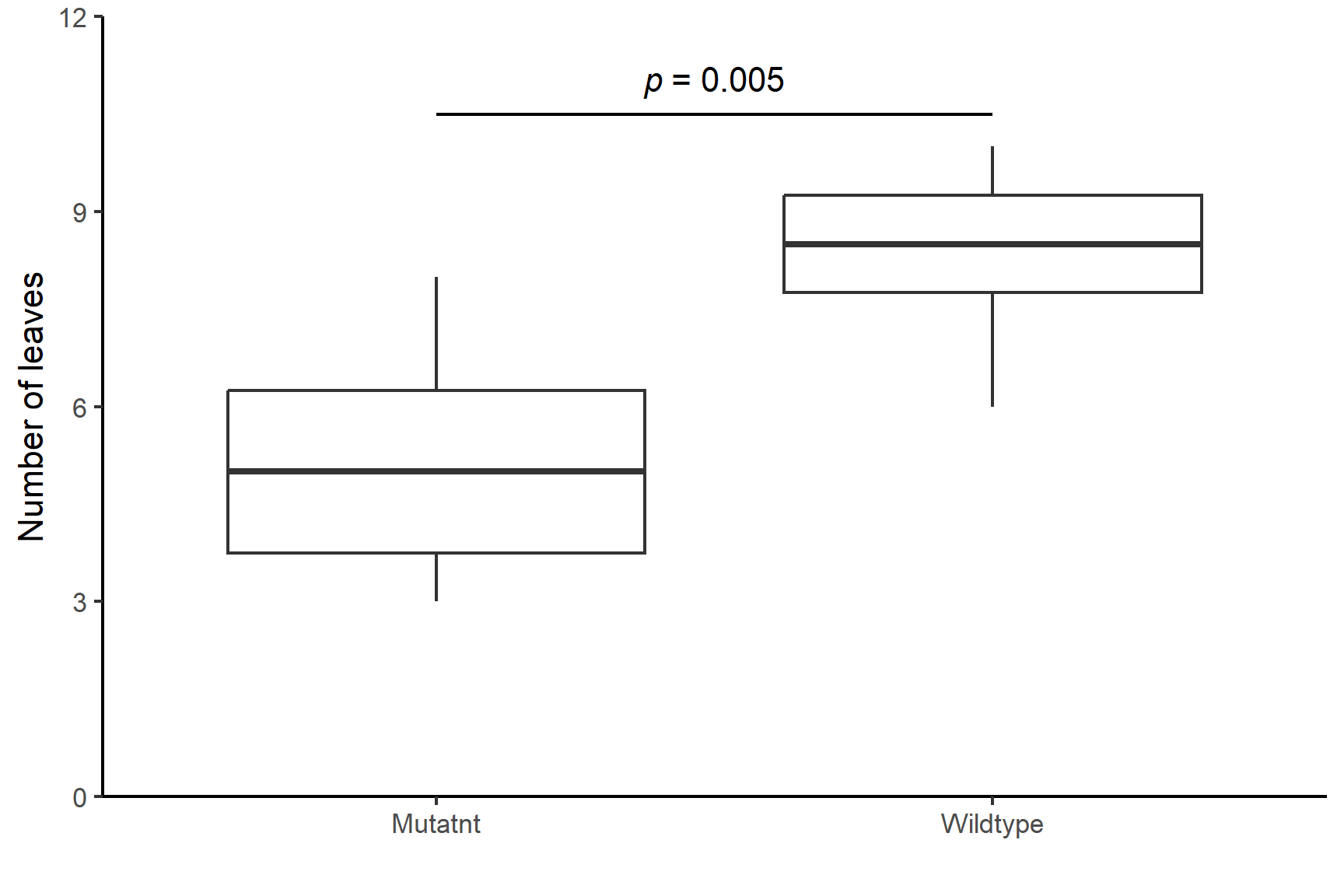

Figure 13.8: Mutant Arabidopsis thaliana have fewer leaves. There are significantly more leaves on wildtype than mutant plants (Wilcoxon rank sum test: W = 5, \(n_1\) = 8, \(n_2\) = 8, p = 0.005). The heavy lines indicate the median of leaves, boxes indicate the interquartile range and whiskers the range. Data analysis was conducted in R (R Core Team 2024) with tidyverse packages (Wickham et al. 2019).

13.5 Two paired-samples, parametric

The data in marks.csv give the marks for ten students in two subjects: Data Analysis and Biology. These data are paired because we have two marks from one student so that a mark in one group has a closer relationship with one of the marks in the other group than with any of the other values. We want to know if students do equally well in both subjects. In this scenario our null hypothesis, \(H_0\), is that there is no difference between the Data Analysis and Biology marks for a student.

13.5.1 Import and explore

Import the data:

marks <- read_csv("data-raw/marks.csv")

Since these data are paired, it makes sense to highlight how the marks differ for each student. One way of doing that is to draw a line linking their marks in each subject. This is known as a spaghetti plot. We can use two geoms: geom_point() and geom_line(). To join a student’s marks, we need to set the group aesthetic to student.¹

ggplot(data = marks, aes(x = subject, y = mark)) +
  geom_point() +
  geom_line(aes(group = student))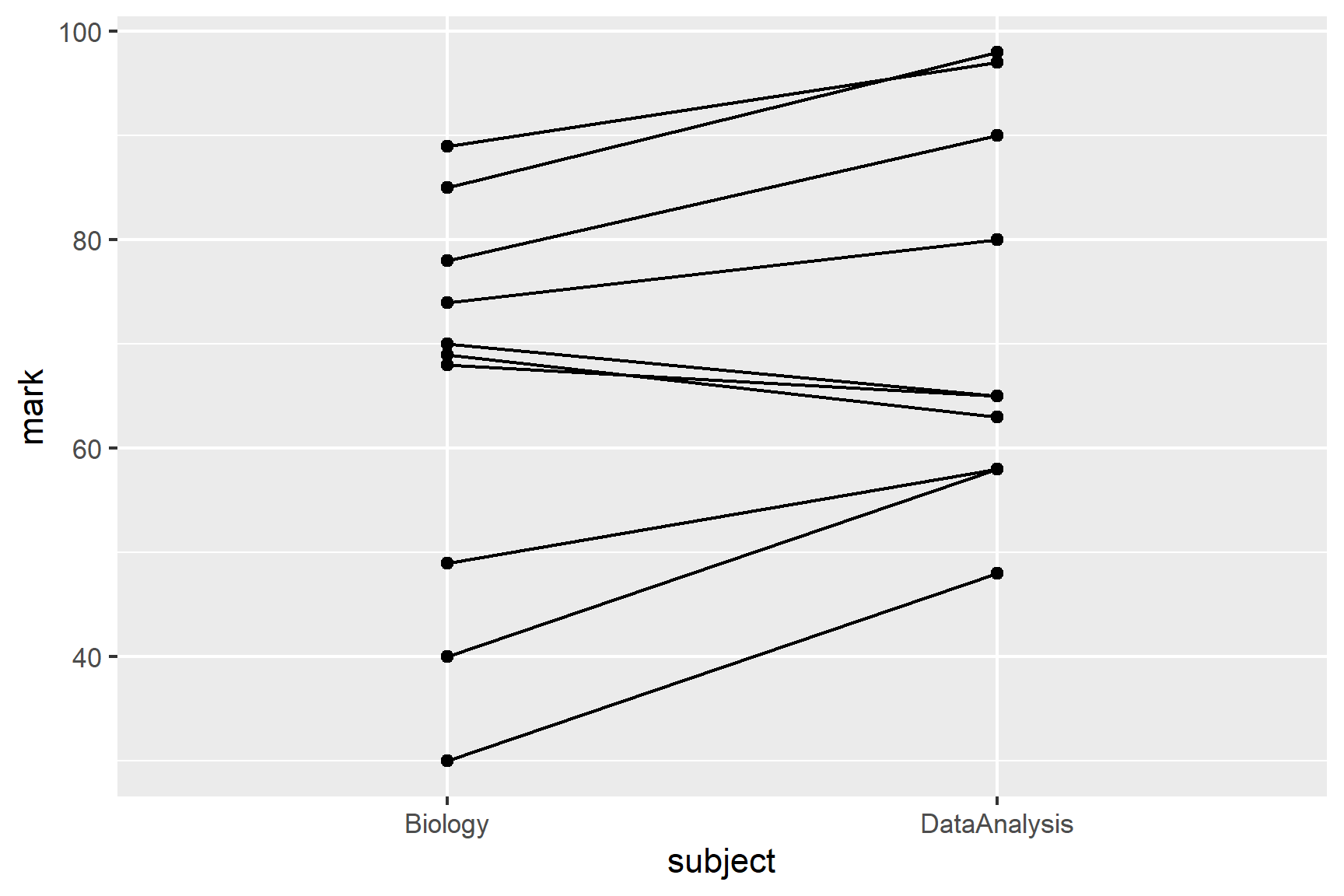

Summarise the data so that we can use the means in plots later:

marks_summary <- marks |>
  group_by(subject) |>
  summarise(mean = mean(mark))

A paired test requires us to into account the variation between students.

13.5.2 Apply lm()

We can create a paired-sample model with the lm() function² like this:

mod <- lm(mark ~ subject + factor(student), data = marks)

• mark is the dependent variable (response).
• subject is the independent variable (explanatory factor).
• factor(student) accounts for the pairing by treating student as another explanatory variable. We have used factor because the values in students are the numbers 1 to 10 and we want student to be treated as a category not a number

summary(mod)
## 
## Call:
## lm(formula = mark ~ subject + factor(student), data = marks)
## 
## Residuals:
##    Min     1Q Median     3Q    Max 
##   -6.5   -3.5    0.0    3.5    6.5 
## 
## Coefficients:
##                     Estimate Std. Error t value Pr(>|t|)    
## (Intercept)           89.500      4.697  19.055 1.39e-08 ***
## subjectDataAnalysis    7.000      2.832   2.471 0.035486 *  
## factor(student)2     -39.500      6.333  -6.237 0.000152 ***
## factor(student)3     -26.500      6.333  -4.184 0.002361 ** 
## factor(student)4     -25.500      6.333  -4.026 0.002990 ** 
## factor(student)5     -16.000      6.333  -2.526 0.032431 *  
## factor(student)6     -54.000      6.333  -8.526 1.33e-05 ***
## factor(student)7      -9.000      6.333  -1.421 0.189010    
## factor(student)8     -27.000      6.333  -4.263 0.002101 ** 
## factor(student)9     -44.000      6.333  -6.947 6.70e-05 ***
## factor(student)10     -1.500      6.333  -0.237 0.818082    
## ---
## Signif. codes:  0 '***' 0.001 '**' 0.01 '*' 0.05 '.' 0.1 ' ' 1
## 
## Residual standard error: 6.333 on 9 degrees of freedom
## Multiple R-squared:  0.9441, Adjusted R-squared:  0.8821 
## F-statistic: 15.21 on 10 and 9 DF,  p-value: 0.0001814

The coefficient for (Intercept) gives the mean Biology mark and that for subjectDataAnalysis is amount that the Data Analysis mark are above Biology marks in general. The p-value tests whether this difference is significantly different from zero. The rest of the output considers how students differ. You can ignore this here.

If you find this a bit overwhelming to read you can use the anova() function on the model object to get a simpler output:

anova(mod)
## Analysis of Variance Table
## 
## Response: mark
##                 Df Sum Sq Mean Sq F value   Pr(>F)    
## subject          1  245.0  245.00   6.108 0.035486 *  
## factor(student)  9 5856.2  650.69  16.222 0.000153 ***
## Residuals        9  361.0   40.11                     
## ---
## Signif. codes:  0 '***' 0.001 '**' 0.01 '*' 0.05 '.' 0.1 ' ' 1

You will notice that the p-value for subject is the same. The test statistic, \(F\) has a value of 6.11and degrees of freedom of 1 and 9. This would be written as $F = $ 6.11; $d.f.= $ 1, 9; $p = $0.035 .

13.5.3 Check assumptions

We might expect marks to be normally distributed. However, this is a very small sample, and choosing a non-parametric test instead would be reasonable. However, we will continue with this example to demonstrate how to interpret and report on the result of a parametric paired-samples test (paired-samples t-test).

A plot the residuals against the fitted values (plot(mod, which = 1)) is not useful for a paired test. The normality of the residuals should be checked.

ggplot(mapping = aes(x = mod$residuals)) +
  geom_histogram(bins = 3)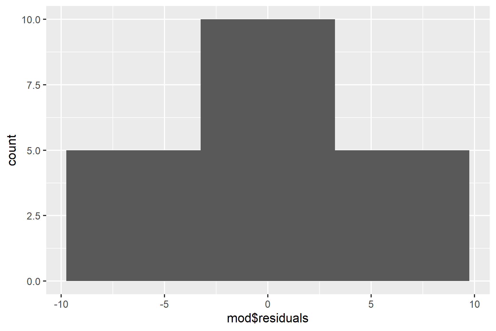

We only have 10 values, so the distribution is never going to look smooth. We can’t draw strong conclusions from this, but we do at least have a peak at 0. Similarly, a normality test is likely to be non-significant because of the small sample size, meaning the test is not very powerful. This means a non-significant result is not strong evidence of the residuals following a normal distribution:

shapiro.test(mod$residuals)
## 
##  Shapiro-Wilk normality test
## 
## data:  mod$residuals
## W = 0.92894, p-value = 0.1473

13.5.4 Report

Individual students score significantly higher in Data Analysis than in Biology (t = 2.47; d.f. = 9; p = 0.0355) with an average difference of 7%. See Figure 13.9

ggplot(data = marks, aes(x = subject, y = mark)) +
  geom_point(pch = 1, size = 3) +
  geom_line(aes(group = student), linetype = 3) +
  geom_point(data = marks_summary,
             aes(x = subject, y = mean),
             size = 3) +
  scale_x_discrete(name = "") +
  scale_y_continuous(name = "Mark",
                     expand = c(0, 0),
                     limits = c(0, 110)) +
  annotate("segment", x = 1, xend = 2,
           y = 105, yend = 105,
           colour = "black") +
  annotate("text", x = 1.5,  y = 108,
           label = expression(italic(p)~"= 0.0355")) +
  theme_classic()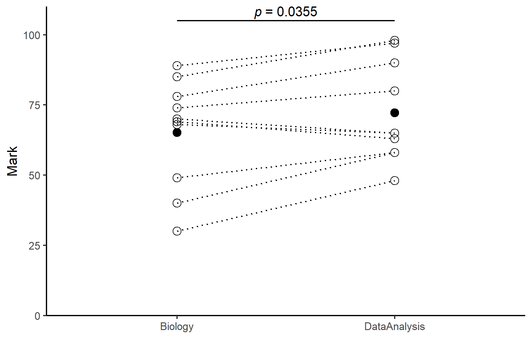

Figure 13.9: Students score higher in Data Analysis than in Biology. Open circles indicate an individual student’s marks in each subject with dashed lines joining their marks in each subject. The filled circles indicate the mean mark for each subject. Individual students score significantly higher in Data Analysis than in Biology (t = 2.47; d.f. = 9; p = 0.0355) with an average difference of 7%. Data analysis was conducted in R (R Core Team 2024) with tidyverse packages (Wickham et al. 2019).

13.6 Two paired-samples, non-parametric

We have the marks for just 10 students. This sample is too small for us to judge whether the marks are normally distributed. We will use a non-parametric test instead. The “Wilcoxon signed-rank” test is the non-parametric equivalent of the paired-samples t-test. This is often referred to as the paired-sample Wilcoxon test, or just the Wilcoxon test.

The test is also applied in R with the wilcox.test() function but we add the paired = TRUE argument. We also have to give the two datasets rather than using the “formula method” of mark ~ subject. This means it is useful to pivot the data to “wide” format.

13.6.1 Pivot wider

Create a new dataframe marks_wide from marks:

marks_wide <- marks |> 
  pivot_wider(values_from = mark, 
              names_from = subject, 
              id_cols = student)

• values_from = mark: Uses the mark column as values in the wide format.
• names_from = subject: Creates new columns based on unique values in subject
• id_cols = student: Keeps student as the identifier (i.e., each row represents a student).

13.6.2 Apply wilcox.test()

To apply a paired test with wilcox.test() we need to use the wide format data (untidy) and add the paired = TRUE argument:

wilcox.test(marks_wide$Biology, marks_wide$DataAnalysis, paired = TRUE)
## 
##  Wilcoxon signed rank test with continuity correction
## 
## data:  marks_wide$Biology and marks_wide$DataAnalysis
## V = 6.5, p-value = 0.03641
## alternative hypothesis: true location shift is not equal to 0

13.6.3 Report

Individual students score significantly higher in Data Analysis than in Biology (Wilcoxon signed rank test: V = 6.5; \(n\) = 10; p = 0.036).

13.7 Summary

1. A linear model with one explanatory variable with two groups and one continuous response is “a two-sample test”.

2. If pairs of observations in the groups have something in common that make them more similar to each other, than to other observations, then those observations are not independent. A paired-samples test is used when the observations are not independent.

3. A linear model with one explanatory variable with two groups and one continuous response is also known as a two-sample t-test when the samples are independent and as a paired-samples t-test when they are not

4. We can use lm() to do two-sample and paired sample tests. We can also use t.test() for these but using lm() helps us understand tests with more groups and/or more variables where we will have to use lm(). The output of lm() is also more typical of the output of statistical functions in R.

5. We estimate the coefficients (also called the parameters) of the model. For a two-sample test these are the mean of the first group, \(\beta_0\) (which might also be called the intercept) and the difference between the means of the first and second groups, \(\beta_1\) (which might also be called the slope). For a paired-sample test there is just one parameter, the mean difference between pairs of values, \(\beta_0\) (which might also be called the intercept). We test whether the parameters differ significantly from zero

6. We can use lm() to a linear regression.

7. In the output of lm() the coefficients are listed in a table in the Estimates column. The p-value for each coefficient is in the test of whether it differs from zero. At the bottom of the output there is a test of the model overall. In this case, this is exactly the same as the test of the \(\beta_1\) and the p-values are identical. The R-squared value is the proportion of the variance in the response variable that is explained by the model.

8. The assumptions of the general linear model are that the residuals are normally distributed and have homogeneity of variance. A residual is the difference between the predicted value and the observed value.

9. We examine a histogram of the residuals and use the Shapiro-Wilk normality test to check the normality assumption. We check the variance of the residuals is the same for all fitted values with a residuals vs fitted plot.

10. If the assumptions are not met, we can use alternatives known as non-parametric tests. These are applied with wilcox.test() in R.

11. When reporting the results of a test we give the significance, direction and size of the effect. Our figures and the values we give should reflect the type of test we have used. We use means and standard errors for parametric tests and medians and interquartile ranges for non-parametric tests. We also give the test statistic, the degrees of freedom (parametric) or sample size (non-parametric) and the p-value. We annotate our figures with the p-value, making clear which comparison it applies to.

R Core Team. 2024. R: A Language and Environment for Statistical Computing. Vienna, Austria: R Foundation for Statistical Computing. https://www.R-project.org/.

Suárez, Nicolás M., Eva Betancor, Tilman E. Klassert, Teresa Almeida, Mariano Hernández, and José J. Pestano. 2009. “Phylogeography and Genetic Structure of the Canarian Common Chaffinch (Fringilla Coelebs) Inferred with mtDNA and Microsatellite Loci.” Molecular Phylogenetics and Evolution 53 (2): 556–64. https://doi.org/10.1016/j.ympev.2009.07.018.

Wickham, Hadley. 2014. “Tidy Data.” Journal of Statistical Software, Articles 59 (10): 1–23. https://vita.had.co.nz/papers/tidy-data.pdf.

Wickham, Hadley, Mara Averick, Jennifer Bryan, Winston Chang, Lucy D’Agostino McGowan, Romain François, Garrett Grolemund, et al. 2019. “Welcome to the Tidyverse” 4: 1686. https://doi.org/10.21105/joss.01686.

Wilcoxon, Frank. 1945. “Individual Comparisons by Ranking Methods.” Biometrics Bulletin 1 (6): 80–83. https://doi.org/10.2307/3001968.

---

1. You might like to try removing aes(group = student) to see what ggplot does when the lines are not grouped by student.

2. This is not the only way to apply a paired test. When there are only two groups and no other explanatory variables, we can use t.test(data = marks, mark ~ subject, paired = TRUE). A more general method that works when you have two or more non-independent values (e.g., more than two subjects) or additional explanatory variables is to create a “linear mixed model” with lmer().